This page is a sub-page of our page on Linear Transformations.
Related KMR pages:
• Representation and reconstruction of linear transformations.
• Setting up a Linear Space Probe for visually exploring linear transformations.
• The Linear War between the planets Vectoria and Vectoria’.
• Singular Values Decomposition.
///////
Related sources of information
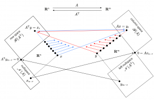
• The Fundamental Theorem of Linear Algebra (by Gilbert Strang)
• Isomorphism Theorems
• Dividing out by the kernel gives (an isomorphism of) the image
///////
The interactive simulations on this page can be navigated with the Free Viewer
of the Graphing Calculator.
///////
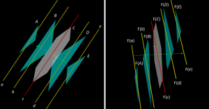
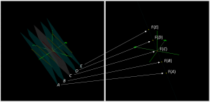
The right part of this figure shows the effect of applying the linear transformation
\, F : {\mathbb{R}}^3 \, \rightarrow \, {\mathbb{R}}^3 \, to the elements shown in the left part. They form the elements of a linear space probe, the structure of which is described here.
Expressed in the standard basis \, S_t \, for \, {\mathbb{R}}^3 , the matrix of \, F \, is given by
[\, F \,]_{S_t}^{S_t} = {\langle \, \begin{matrix} 1 & 1 & 1 \\ 1 & -1 & h \\ 2 & 0 & 2 \end{matrix} \, \rangle}_{S_t}^{S_t} = \begin{bmatrix} 1 & 1 & 1 \\ 1 & -1 & h \\ 2 & 0 & 2 \end{bmatrix} .
NOTE: Our use of vertical braces (as on the right-hand side) to denote the matrix of a linear transformation – expressed in the standard bases for its domain and its codomain – is inconsistent with our general notation for representation, which, in the case of representing a linear map with respect to a basis of its domain and a basis of its codomain, is expressed as:
[l_{inearMap}]_{B_{asisOfCodomain}}^{B_{asisOfDomain}} = \left< \, m_{atrix} \, \right>_{B_{asisOfCodomain}}^{B_{asisOfDomain}} .
This notation uses vertical braces (as on the left-hand side) to denote the representation of a representee with respect to a basis. Hence, in the above formula, the \, l_{inearMap} \, is the \, r_{epresentee} \, and the \, m_{atrix} \, is the \, r_{epresentation} .
However, this notational inconsistency is more of a nuisance than a problem, since the relevant bases for the domain and the codomain of \, F \, are most often clear from the computational context. Moreover, this inconsistency has the benefit of making our notation for matrices compatible with the mainstream notation of matrix algebra, where matrices can be considered as computational objects in themselves – and also as representations of many other types of constructs besides linear transformations.
///////
Linear map \, F = ((1 ,1, 1) , (1, -1, h), (2, 0, 2)), h = 0 \implies \det F = 2(h-1) = -2 \ne 0 \implies \textnormal{rank} \, F = 3 , (rotating planes):
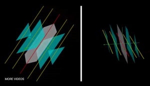
In the left window, this video shows the parallel planes of the space probe rotating “in parallel with” the central plane (in grey), which, in turn, is rotating around the central line (in red). The right window shows the effect of applying the linear map \, F \, to the elements shown in the left window.
Since \, F \, is a linear map, \, F \, it is also an affine map,
that is, a composition of a translation and a linear map.
Because affine maps preserve parallelism of linear elements,
parallel planes and lines of the space probe are mapped by \, F \, into parallel elements.
The rank of a linear transformation is the dimension of its image space, which is a linear subspace of its codomain.
The codomain of any transformation is the “target space” that the transformation is mapping each element of its domain to. In the case of a linear transformation, both the domain and the codomain are linear spaces (= vector spaces) and the elements of these spaces are the vectors that “live” in them.
Hence, for the linear transformation \, F : {\mathbb{R}}^3 \, \rightarrow \, {\mathbb{R}}^3 \, we have:
• \,\, \textnormal{rank} \, F = \dim(\textnormal{im} \, F) .
• \,\, \textnormal{im} \, F \, is a linear subspace of the linear space \, \textnormal{codomain} \, F \, which is equal to \, {\mathbb{R}}^3 .
The case of full rank (rank F = 3)
A linear map \, F \, has full rank if and only if the column-vectors of the matrix for \, F \, are linearly independent. This means that the images under \, F \, of the basis-vectors of the domain of \, F \, span as large a subspace of the codomain of \, F \, as they possibly can.
Because the map \, F \, is affine, the parallel planes of the space probe are mapped into “image planes” that are still parallel. Moreover, since \, F \, has full rank, the image of \, F \, is the entire \, {\mathbb{R}}^3 , i.e., we have \, \textnormal{im} \, F = \textnormal{codomain} \, F .
Hence the image planes of the light-blue planes of the space probe NEVER coincide with the same plane, no matter how we rotate the planes since, if they did coincide, the mapping could NOT have full rank. This full-rank configuration can be observed in the following screenshot from the video above:
An endomorphism is a transformation from a space to itself. A linear endomorphism \, F : V \rightarrow V \, is represented by a quadratic matrix of format \, n \, \textnormal{x} \, n \, , where \, n = \dim V \, is the dimension of the vector space \, V .
For a quadratic matrix, full rank is equivalent to zero null-space. This is a consequence of the rank-nullity theorem of linear algebra, which implies that if a linear endomorphism \, F \, , i.e., a linear map \, F : V \rightarrow V , has full rank, then its null-space \, \ker \, F \, must be zero.
In its general form, the rank-nullity theorem can be expressed as:
\, \dim(\ker \, F) + \dim(\textnormal{im} \, F) = \dim(\textnormal{domain} \, F) .
The rank-nullity theorem is part of the fundamental theorem of linear algebra. The intuitive meaning of the rank-nullity theorem is that if we add the dimension of the null-space of \, F \, , i.e., the subspace \, \ker \, F \, of the domain of \, F \, that is mapped to zero, and the dimension of \, \textnormal{im} \, F \, , i.e., the dimension of the space that “is left” after we have applied the linear transformation \, F , then the result is the dimension of \, \textnormal{domain} \, F \, , i.e., the dimension of the space that we had “at the beginning,” before we applied \, F .
In words: Let \, F : {\mathbb{R}}^m \, \rightarrow \, {\mathbb{R}}^n \, be a linear transformation. Then
The dimension of \, \ker F , which is the linear subspace that is mapped to zero,
plus the dimension of \, \textnormal{im} \, F , which is the linear subspace that is left,
is equal to the dimension of \, \textnormal{domain} \, F , which is the linear space that we started with .
///////
The case of rank F = 2
We will now study what it looks like when the rank of \, F \, decreases from three to two.
This situation corresponds to \, \det F = 0 , and, since the matrix of \, F \, in the standard basis is given by
[\, F \,]_{S_t}^{S_t} = \begin{bmatrix} 1 & 1 & 1 \\ 1 & -1 & h \\ 2 & 0 & 2 \end{bmatrix} ,
we have \, \det F \equiv 2(h - 1) \, and hence \, \det F = 0 \, \iff \, h = 1 .
Linear map \, F = ((1 ,1, 1) , (1, -1, h), (2, 0, 2)), 0 \le h \le 2, h = 1 \implies \textnormal{rank} \, F = 2 \, , (fixed lines and planes):
///////
Linear map \, F = ((1 ,1, 1) , (1, -1, 1), (2, 0, 2)), \textnormal{rank} \, F = 2 \, ,
(rotating planes):
///////
Linear map \, F = ((1 ,1, 1) , (1, -1, h), (2, 0, 2)), 0 \le h \le 2, h = 1 \implies \textnormal{rank} \, F = 2 \, , (rotating lines):
///////
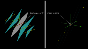
The kernel and the image of the rank 2 linear map F = ((1 ,1, 1) , (1, -1, 1), (2, 0, 2)):
///////
\, \begin{bmatrix} 1 & 1 & 1 \\ 1 & -1 & 1 \\ 2 & 0 & 2 \end{bmatrix} \begin{bmatrix} x \\ y \\ z \end{bmatrix} = \begin{bmatrix} 0 \\ 0 \\ 0 \end{bmatrix} \, implies
\, x \begin{bmatrix} 1 \\ 1 \\ 2 \end{bmatrix} + y \begin{bmatrix} 1 \\ -1 \\ 0 \end{bmatrix} + z \begin{bmatrix} 1 \\ 1 \\ 2 \end{bmatrix} = \begin{bmatrix} 0 \\ 0 \\ 0 \end{bmatrix} \, \implies \, z = -x \, and \, y = 0 .
Hence we have:
The nullspace of \, F \, : \, \mathscr{N}(F) = \{ \, \lambda \begin{bmatrix} 1 \\ 0 \\ -1 \end{bmatrix} \, | \; \lambda \in \mathbb{R} \, \} .
Moreover, since the first and the third columns of \, F \, are equal, we have:
The column space of \, F \, : \, \mathscr{R}(F) = \{ \, \alpha \begin{bmatrix} 1 \\ 1 \\ 2 \end{bmatrix} + \beta \begin{bmatrix} 1 \\ -1 \\ 0 \end{bmatrix} \, | \; \alpha, \beta \in \mathbf {R} \, \} .
///////
The case of rank F = 1
In order to achieve a rank 2 into rank 1 collapse, we will change the matrix for \, F \, in comparison to the simulations above:
Expressed in the standard basis \, S_t \, for \, {\mathbb{R}}^3 , the matrix for the \, F \, that we will use is given by:
[\, F \,]_{S_t}^{S_t} = {\langle \, \begin{matrix} 1 & 1 & 1 \\ 1 & 1 & h \\ 1 & 1 & 1 \end{matrix} \, \rangle}_{S_t}^{S_t} = \begin{bmatrix} 1 & 1 & 1 \\ 1 & 1 & h \\ 1 & 1 & 1 \end{bmatrix} .
Linear map \, F = ((1 ,1, 1) , (1, 1, h), (1, 1, 1)), 0 \le h \le 2 \,
\, h = 1 \implies \textnormal{rank} \, F = 1 \,
Linear map \, F = ((1 ,1, 1) , (1, 1, 1), (1, 1, 1)), \textnormal{rank} \, F = 1 :
The kernel and the image of the rank 1 linear map \, F = ((1 ,1, 1) , (1, 1, 1), (1, 1, 1)):
///////
\, \begin{bmatrix} 1 & 1 & 1 \\ 1 & 1 & 1 \\ 1 & 1 & 1 \end{bmatrix} \begin{bmatrix} x \\ y \\ z \end{bmatrix} = \begin{bmatrix} x + y + z \\ x + y + z \\ x + y + z \end{bmatrix} = (x + y + z) \begin{bmatrix} 1 \\ 1 \\ 1 \end{bmatrix} .
///////
The nullspace of a linear map is perpendicular to the image space of its transpose
\, \ker A \perp \image A^{T} \, and \, \ker A^T \perp \image A \, .
///////
