This page is a sub-page of our page on Matrices and Gaussian Elimination.
///////
Related KMR-pages:
• Matrix Algebra
• Linear Algebra
• The Rank-Nullity Theorem
///////
Related sources of information:
• Strang, Gilbert (1986), Linear Algebra and its Applications, Third Edition (1988).
///////
/////// Quoting Strang (1986, p. 71)
The elimination process is by now very familiar for square matrices, and one example will be enough to illustrate the new possibilities when the matrix is rectangular. The elimination itself goes forward without major changes, but when it comes to reading off the solution by back-substitutions, there are some differences.
Perhaps, even before the example, we should illustrate the possibilities by looking at the scalar equation \, a x = b . This is a “system” of only one equation in one unknown. It might be \, 3 x = 4 \, or \, 0 x = 0 \, or \, 0 x = 4 , and those examples display the three alternatives.
(i) If \, a \neq 0 , then for any \, b \, there exists a solution \, x = b/a , and this solution is unique. This is the nonsingular case (of a 1 by 1 invertible matrix \, a ).
(ii) If \, a = 0 \, and \, b = 0 , there are infinitely many solutions; any \, x \, satisfies \, 0 x = 0 . This is the underdetermined case; a solution exists, but it is not unique.
(iii) If \, a = 0 \, and \, b \neq 0 , there is no solution to \, 0 x = b . This is the inconsistent case.
For square matrices all these alternatives may occur. We will replace “ a = 0 ” by “ A \, is invertible,” but it still means that \, A^{-1} \, makes sense. With a rectangular matrix possibility (i) disappears; we cannot have existences and also uniqueness, one solution \, x \, for every \, b . There may be infinitely many solutions for every \, b ; or infinitely many for some \, b \, and no solutions for others; or one solution for some \, b \, and none for others.
We start with a 3 by 4 matrix, ignoring at first the right side \, b \, :
\, A = \begin{bmatrix} 1 & 3 & 3 & 2 \\ 2 & 6 & 9 & 5 \\ -1 & -3 & 3 & 0 \end{bmatrix} .
The pivot \, a_{11} = 1 \, is nonzero, and the usual elementary operations will produce zeros in the first columns below this pivot:
\, A \rightarrow \begin{bmatrix} 1 & 3 & 3 & 2 \\ 0 & 0 & 3 & 1 \\ 0 & 0 & 6 & 2 \end{bmatrix} .
The candidate for the second pivot has become zero, and therefore we look below it for a nonzero entry – intending to carry out a row exchange. In this case the entry below it is also zero. If the original matrix were square, this would signal that the matrix was singular. With a rectangular matrix, we must expect trouble anyway, and there is no reason to terminate the elimination. All we can do is to go on to the next column, where the pivot entry is nonzero. Subtracting twice the second row from the third, we arrive at
\, U = \begin{bmatrix} 1 & 3 & 3 & 2 \\ 0 & 0 & 3 & 1 \\ 0 & 0 & 0 & 0 \end{bmatrix} .
Strictly speaking, we then proceed to the fourth column; there we meet another zero in the pivot position, and nothing can be done. The forward stage of elimination is complete.
The final form \, U \, is again upper triangular, but the pivots are not necessarily on the main diagonal. The important thing is that the nonzero entries are confined to a “staircase pattern,” or echelon form which is indicated in a 5 by 9 case by Fig. 2.2. The pivots are circled, whereas the other starred entries may or may not be zero.
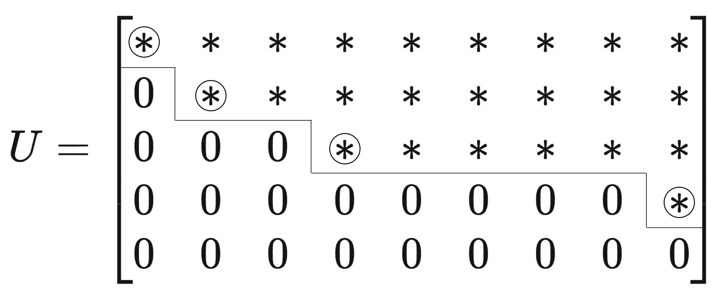
We can summarize in words what the figure illustrates:
(i) The nonzero rows come first – otherwise there would have been row exchanges
– and the pivots are the first nonzero entries in those rows.
(ii) Below each pivot is a column of zeros, obtained by elimination.
(iii) Each pivot lies to the right of the pivot in the row above;
this produces the staircase pattern.
Since we started with \, A \, and ended with \, U , the reader is certain to ask:
Are these matrices connected by a lower triangular \, L \, as before? Is \, A = L U \, ?
There is no reason why not, since the elimination steps have not changed; each step still subtracts a multiple of one row from a row beneath it. The inverse of each step is also accomplished just as before, by adding back the multiple that was subtracted.
These inverses still come in an order that permits us to record them directly in \, L \, :
\, L = \begin{bmatrix} 1 & 0 & 0 \\ 2 & 1 & 0 \\ -1 & 2 & 1 \end{bmatrix} .
The reader can verify that \, A = L U , and should note that \, L \, is not rectangular but square. It is a matrix of the same order \, m = 3 \, as the number of rows in \, A \, and \, U .
The only operation not required by our example, but needed in general, is an exchange of rows. As in Chapter 1, this would introduce a permutation matrix \, P \, and it can carry out row exchanges before elimination begins. Since we keep going to the next column when no pivots are available in a given column, there is no need to assume that \, A \, is nonsingular.
Here is the main theorem:
2B To any \, m \, by \, n \, matrix \, A \, there correspond a permutation matrix \, P , a lower triangular matrix \, L \, with unit diagonal, and an \, m \, by \, n \, echelon matrix \, U \, , such that \, P A = L U .
Our goal is now to read off the solutions (if any) to \, A x = b .
Suppose we start with the homogeneous case, \, b = 0 . Then, since the row operations will have no effect on the zeros on the right side of the equation, \, A x = 0 \, is simply reduced to \, U x = 0 \, :
\, U x = \begin{bmatrix} 1 & 3 & 3 & 2 \\ 0 & 0 & 3 & 1 \\ 0 & 0 & 0 & 0 \end{bmatrix} \begin{bmatrix} u \\ v \\ w \\ y \end{bmatrix} = \begin{bmatrix} 0 \\ 0 \\ 0 \end{bmatrix} .
The unknowns \, u, v, w, \, and \, y \, go into two groups:
One group is made up of the basic variables, corresponding to columns with pivots.
The first and third columns contain the pivots, so \, u \, and \, w \, are the basic variables.
The other group is made up of the free variables, corresponding to columns without pivots; these are the second and fourth columns, so that \, v \, and \, y \, are free variables.
To find the most general solution to \, U x = 0 \, (or equivalently, to \, A x = 0 ) we may assign arbitrary values to the free variables. Suppose we call these values simply \, v \, and \, y . The basic variables are then completely determined, and can be computed in terms of the free variables by back-substitution. Proceeding upward,
\, 3w + y = 0 \, yields \, w = - \tfrac{1}{3} y \,
\, u + 3v + 3w + 2y = 0 \, yields \, u = -3v - y .
There is a “double infinity” of solutions to the system, with two free and independent parameters \, v \, and \, y . The general solution is a combination
\, x = \begin{bmatrix} -3v - y \\ v \\ - \tfrac{1}{3} y \\ y \end{bmatrix} = v \begin{bmatrix} -3 \\ 1 \\ 0 \\ 0 \end{bmatrix} + y \begin{bmatrix} -1 \\ 0 \\ - \tfrac{1}{3} \\ 1 \end{bmatrix} .
Please look again at the last form of the solution to \, A x = b . The vector \, (-3, 1, 0, 0) gives the solution when the free variables have the values \, v = 1, y = 0 . The last vector is the solution when \, v = 0 \, and \, y = 1 . All solutions are linear combinations of these two. Therefore a good way to find all solutions to \, A x = 0 \, is
1. After elimination reaches \, U x = 0 , identify the basic and the free variables.
2. Give one free variable the value one, set the other free variables to zero, and solve \, U x = 0 \, for the basic variables.
3. Every free variable produces its own solution by step 2, and the combinations of those solutions form the nullspace – the space of all solutions to \, A x = 0 .
Geometrically, the picture is this: Within the four-dimensional space of all possible vectors \, x , the solutions to \, A x = 0 \, form a two-dimensional subspace – the nullspace of \, A . In the example it is generated by the two vectors \, (-3, 1, 0, 0) \, and \, (-1, 0, -\tfrac{1}{3}, 1) . The combinations of these two vectors form a set that is closed under addition and scalar multiplication; these operations simply lead to more solutions to \, A x = 0 , and all these combinations comprise the nullspace.
This is the place to recognize one extremely important theorem. Suppose we start with a matrix that has more columns than rows, \, n > m . Then, since there can be at most \, m \, pivots (there are not rows enough to hold any more), there must be at least \, n - m \, free variables. There will be even more free variables if some rows of \, U \, happen to reduce to zero; but no matter what, at least one of the variables must be free. This variable can be assigned an arbitrary value, leading to the following conclusion:
2C If a homogeneous system \, A x = 0 \, has more unknowns than equations ( n > m ), then it has a nontrivial solution: There is a solution \, x \, other than the trivial solution \, x = 0 .
There must actually be infinitely many solutions, since any multiple \, c x \, will also satisfy \, A (c x) = 0 . The nullspace contains the line through \, x . And if there are additional free variables, the nullspace becomes more than just a line in \, n -dimensional space. The nullspace is a subspace of the same “dimension” as the number of free variables.
The central idea – the dimension of a subspace – is made precise in the next section. It is a count of the degrees of freedom.
The inhomogeneous case, \, b \neq 0 , is quite different. We return to the original example \, A x = b , and apply to both sides of the equation the operations that led from \, A \, to \, U . The result is an upper triangular system \, U x = c \, :
\, \begin{bmatrix} 1 & 3 & 3 & 2 \\ 0 & 0 & 3 & 1 \\ 0 & 0 & 0 & 0 \end{bmatrix} \begin{bmatrix} u \\ v \\ w \\ y \end{bmatrix} = \begin{bmatrix} b_1 \\ b_2 - 2 b_1 \\ b_3 - 2 b_2 + 5 b_1 \end{bmatrix} .
The vector \, c \, on the right side, which appeared after the elimination steps ,is just \, L^{-1} b \, as in the previous chapter.
It is not clear that these equations have a solution. The third equation is very much in doubt. Its left side is zero and the equations are inconsistent unless \, b_3 - 2 b_2 + 5 b_1 = 0 . In other words, the set of attainable vectors b is not the whole of three-dimensional space. Even though there are more unknowns than equations, there may be no solution. We know, from Section 2.1, another way of considering the same question: A x = b can be solved if and only if b lies in the column space of \, A . This subspace is spanned by the four columns of \, A \, (not of \, U !):
\, \begin{bmatrix} 1 \\ 2 \\ -1 \end{bmatrix}, \;\;\;\; \begin{bmatrix} 3 \\ 6 \\ -3 \end{bmatrix}, \;\;\;\; \begin{bmatrix} 3 \\ 9 \\ 3 \end{bmatrix}, \;\;\;\; \begin{bmatrix} 2 \\ 5 \\ 0 \end{bmatrix} .
Even though there are four vectors, their combinations only fill out a plane in three-dimensional space. The second column is three times the first, and the fourth column equals the first plus some fraction of the third. (Note that these dependent columns, the second and fourth, are exactly the columns without pivots.) The column space can now be described in two completely different ways. On the one hand, it is the plane generated by the columns 1 and 3; the other columns lie in that plane, and contribute nothing new. Equivalently, it is the plane composed of all points \, (b_1, b_2, b_3) \, that satisfy \, b_3 - 2 b_2 + 5 b_1 = 0 ; this is the constraint that must be imposed if the system is to be solvable. Every column satisfies this constraint, so it is forced on \, b . Geometrically, we shall see that the vector \, (5, -2, 1) \, is perpendicular to each column.
If \, b \, lies in this plane, and thus belongs to the column space, then the solutions of \, A x = b \, are easy to find. The last equation in the system amounts only to \, 0 = 0 . To the free variables \, v \, and \, y , we may assign arbitrary values as before. Then the basic variables are still determined by back-substitution. We take a specific example, in which the components of \, b \, are chosen as \, 1, 5, 5 \, (we were careful to make \, b_3 - 2 b_2 + 5 b_1 = 0 ). The system \, A x = b \, becomes
\, \begin{bmatrix} 1 & 3 & 3 & 2 \\ 2 & 6 & 9 & 5 \\ -1 & -3 & 3 & 0 \end{bmatrix} \begin{bmatrix} u \\ v \\ w \\ y \end{bmatrix} = \begin{bmatrix} 1 \\ 5 \\ 5 \end{bmatrix} .
Elimination converts this into
\, \begin{bmatrix} 1 & 3 & 3 & 2 \\ 0 & 0 & 3 & 1 \\ 0 & 0 & 0 & 0 \end{bmatrix} \begin{bmatrix} u \\ v \\ w \\ y \end{bmatrix} = \begin{bmatrix} 1 \\ 3 \\ 0 \end{bmatrix} .
The last equation is \, 0 = 0 , as expected, and the others give
\, 3 w + y = 3 \;\;\;\;\; or \;\;\;\;\; w = 1 - \tfrac{1}{3} y
\, u + 3 v + 3 w + 2 y = 1 \;\;\;\;\; or \;\;\;\;\; u = -2 - 3 v - y .
Again, there is a double infinity of solutions. Looking at all four components together, the general solution can be written as
\, x = \begin{bmatrix} u \\ v \\ w \\ y \end{bmatrix} = \begin{bmatrix} -2 \\ 0 \\ 1 \\ 0 \end{bmatrix} + v \begin{bmatrix} -3 \\ 1 \\ 0 \\ 0 \end{bmatrix} + y \begin{bmatrix} -1 \\ 0 \\ -\tfrac{1}{3} \\ 1 \end{bmatrix} .
This is exactly as the solution to \, A x = 0 \, in equation (1), except there is one new term. It is \, (-2, 0, 1, 0) , which is a particular solution to \, A x = b . It solves the equation, and then the last two terms yield more solutions (because they satisfy \, A x = 0 ).
Every solution to \, A x = b \, is the sum of one particular solution and a solution to \, A x = 0 \, :
\, x_{general} = x_{particular} + x_{homogeneous} \,
The homogeneous part comes from the nullspace. The particular solution in (3) comes from solving the equation with all free variables set to zero. That is the only new part, since the nullspace is already computed. When you multiply the equation above by \, A , you get
\, A x_{general} = b + 0 .
Geometrically, the general solutions again fill a two-dimensional surface – but it is not a subspace. It does not contain the origin. It is parallel to the nullspace [*] we had before, but it is shifted by the particular solution. Thus the computations include one new step:
1. Reduce \, A x = b \, to \, U x = c .
2. Set all free variables to zero and find a particular solution.
3. Set the right side to zero and give each free variable, in turn, the value one. With the other free variables at zero, find a homogeneous solution (a vector \, x \, in the nullspace).
Previously step 2 was absent. When the equation was \, A x = 0 , the particular solution was the zero vector! It fits the pattern, but \, x_{particular} = 0 \, was not printed in equation (1). Now it added to the homogeneous solutions, as in (3).
/////////////////////////////////// Interrupting the quote from Strang (1986).
[*]: In fact, it is an affine subspace, which is a linear subspace that has been “parallel-shifted” (= translated) away from “passing through the origin”. More on affine geometry at the KMR web site.
/////////////////////////////////// Continuing the quote from Strang (1986):
Elimination reveals the number of pivots and the number of free variables. if there are \, r \, pivots, there are \, r \, basic variables and \, n - r \, free variables. That number \, r \, will be given a name – it is the rank of the matrix – and the whole elimination process can be summarized:
2D Suppose elimination reduces \, A x = b \, to \, U x = c . Let there be \, r \, pivots; the last \, m - r \, rows of \, U \, are zero. Then there is a solution only if the last \, m - r \, components of \, c \, are all zero. If \, r = m , there is always a solution.
The general solution is the sum of a particular solution (with all free variables zero) and a homogeneous solution (with the \, n - r \, free variables as independent parameters).
If \, r = n , there are no free variables and the nullspace contains only \, x = 0 .
The number \, r \, is called the rank of the matrix \, A .
Note the two extreme cases, when the rank is as large as possible:
(1) If \, r = n , there are no free variables in \, x .
(2) If \, r = m , there are no zero rows in \, U .
With \, r = n \, the nullspace contains only \, x = 0 . The only solution is \, x_{particular} .
With \, r = m \, there are no constraints on \, b , the column space is all of \, \mathbf{R}^m , and
for every right-hand side the equation can be solved.
/////// End of quote from Strang (1986)