This page is a sub-page of our page on Geometry.
Related KMR pages:
• The Rank-Nullity theorem
• Affine approximation
• A Linear Space Probe
///////
Other relevant sources of information:
• Affine geometry
• Rigid-body transformations in a plane (2D)
• Snapper E. and Troyer, R. J., (1971): Metric Affine Geometry, Dover, 1989.
///////
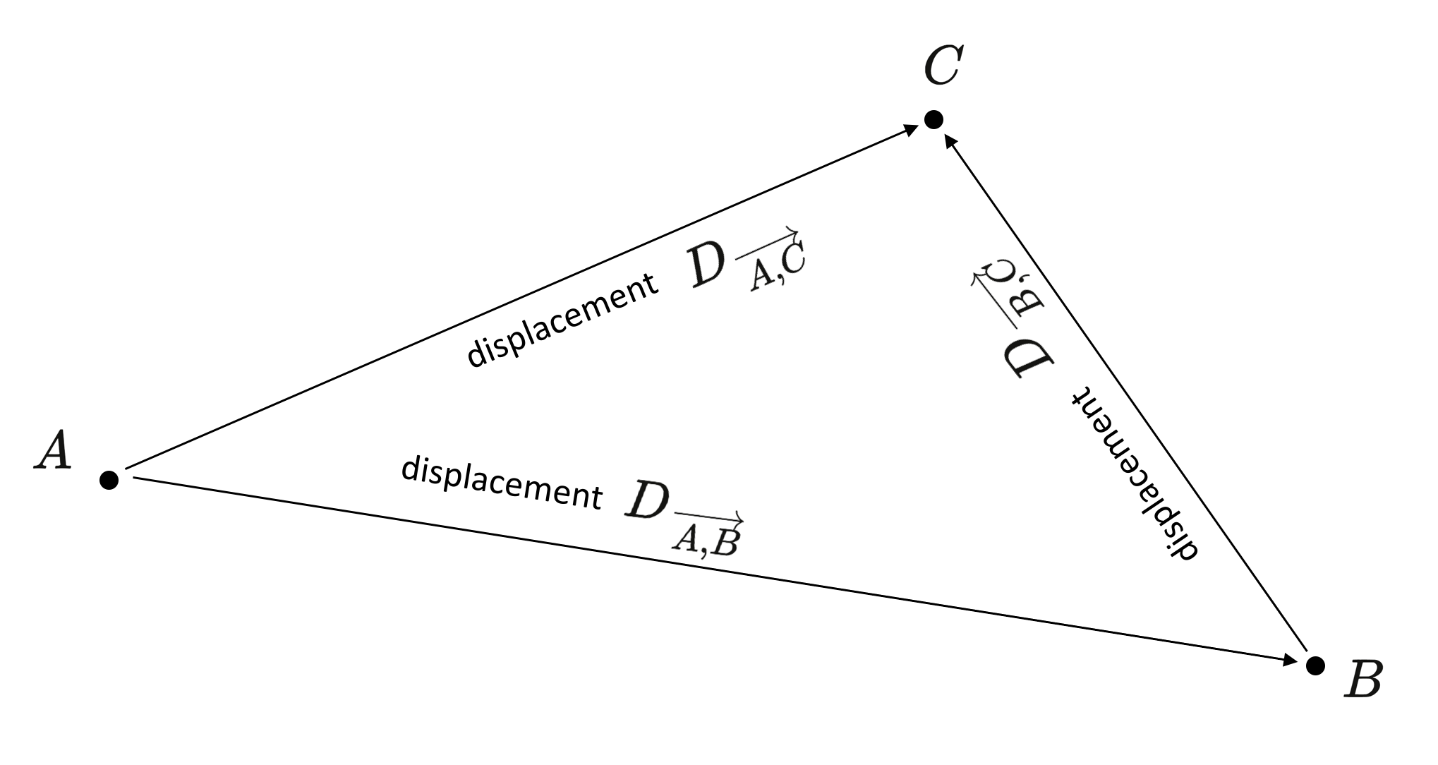
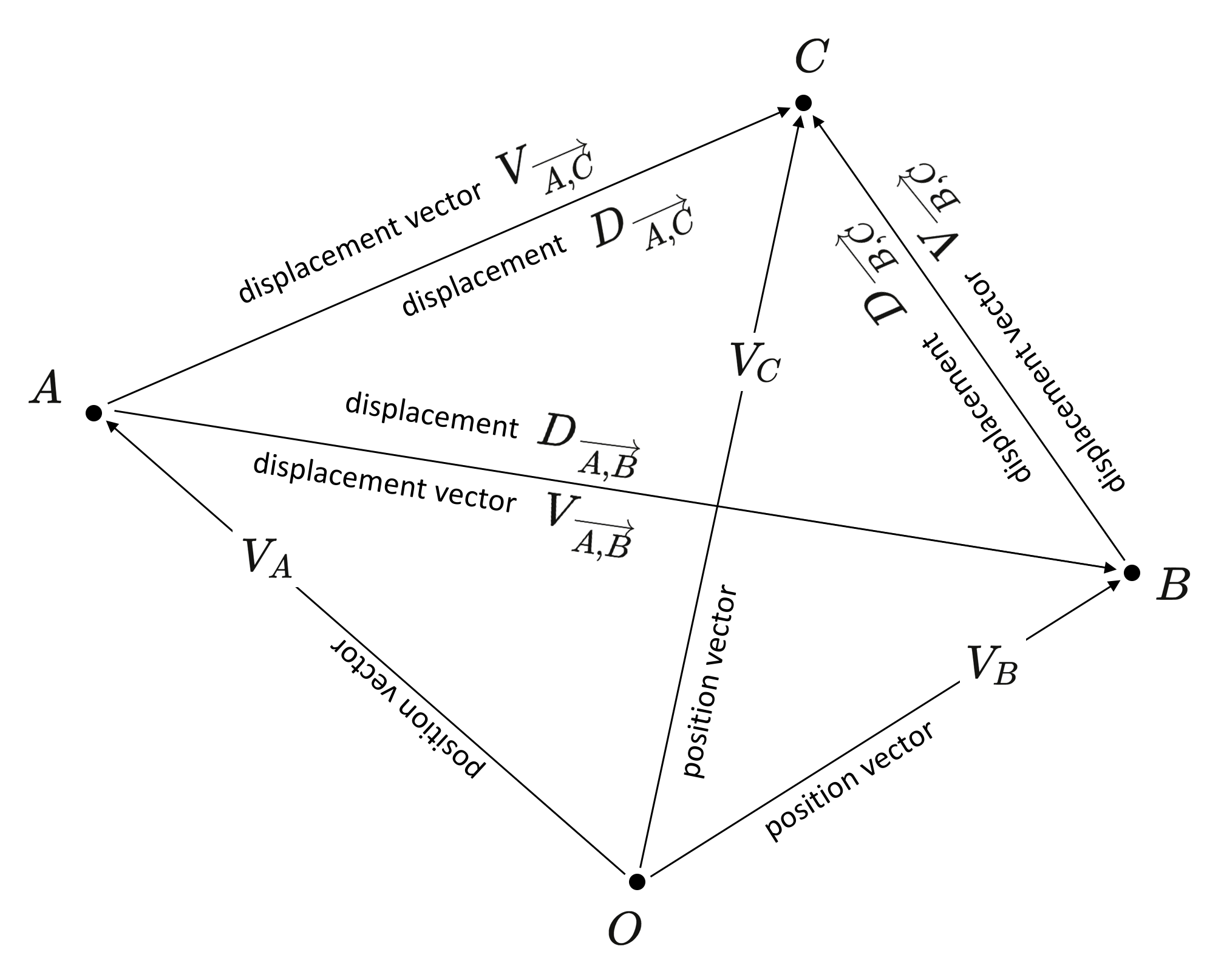
\, \overrightarrow {x ,A x} \, \, D_{\, \overrightarrow {A ,B}} \, D_{\, \overrightarrow {B ,C}} \, D_{\, \overrightarrow {A ,C}} \, \, V_{\, \overrightarrow {A ,B}} \, V_{\, \overrightarrow {B ,C}} \, V_{\, \overrightarrow {A ,C}} \, \, V_A \, V_B \, V_C \, A \, B \, C \, O \, \, D_{\, \overrightarrow {A ,B}}(A) = B \;\;, \;\; D_{\, \overrightarrow {B ,C}}(B) = C \, D_{\, \overrightarrow {B ,C}} (D_{\, \overrightarrow {A ,B}}(A)) \, = \, D_{\, \overrightarrow {A ,B} + \overrightarrow {B ,C}} (A) = D_{\, \overrightarrow {A ,C}} (A) = C \, \, D_{\, \overrightarrow {A ,B}} (D_{\, \overrightarrow {B ,C}}(A)) \, = \, D_{\, \overrightarrow {B ,C} + \overrightarrow {A ,B}} (A) = D_{\, \overrightarrow {A ,C}} (A) = C \,///////
Positions and their Displacements:
///////
Positions and Displacements – and their representations as
position vectors and displacement vectors:
Position vector: \, {[ \, A \, ]}_O \, = \, {\langle \, V_A \, \rangle}_O \,
Displacement vector: \, {[ \, D_{\overrightarrow {A, B}} \, ]}_O \, = \, {\langle \, V_{\overrightarrow {A, B}} \, \rangle}_O \,
Position vector + Displacement vector = Position vector: \, V_A + V_{\overrightarrow {A, B}} = V_B \,
///////
/////// Quoting Snapper and Troyer (1971, p. 1):
1. INTUITIVE AFFINE GEOMETRY
Our subject is geometry and we shall begin with the study of affine geometry. To follow a more historical order, we would begin with Euclidean geometry. However, it seems useful to separate the axioms of affine geometry from those of Euclidean geometry. Roughly speaking, affine geometry is what remains after practically all ability to measure length, area, angles, etc., has been removed from Euclidean geometry. One might think that affine geometry is a poverty-stricken subject. On the contrary, affine geometry is quite rich. Even after almost all ability to measure has been removed from Euclidean geometry, there still remains the concept of parallelism. Consequently, the whole theory of homothetic figures lies within affine geometry. The notions of translation and magnification (these are the dilations or similarities) are in the domain of affine geometry and, more generally, as the name suggests, affine transformations (one-to-one, onto functions which preserve parallelism) constitute an affine notion.
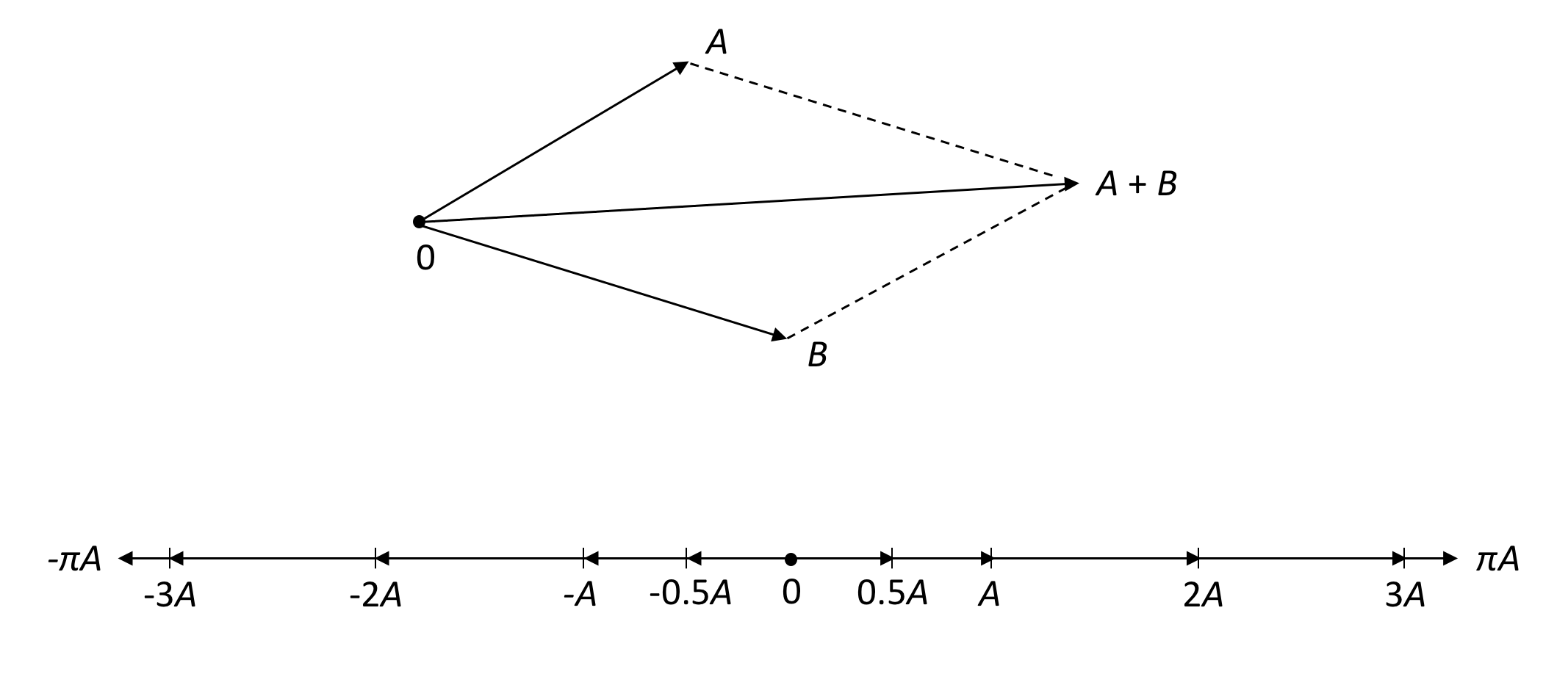
The question of how to obtain a rigorous approach to affine geometry arises. We choose to base our axiom system on linear algebra, that is, on the theory of vector spaces. First, let us discuss, on an intuitive level, the connection between plane affine geometry and vector spaces. What is the intuitive notion of the affine plane \, P \, over the field of real numbers? The points of \, P \, can be viewed as the points of any physical plane. If we fix a particular point \, 0 \, of \, P , we can construct a vector space in a natural way. The vectors are the ordered pairs \, (0, A) \, where \, A \in P \, and we picture such a vector as an arrow from \, 0 \, to \, A \, , see Figure 2.1:

We often write \, A \, for the vector \, (0, A) , but this can only be done if it is clear from the context which point is being used as \, 0 , that is, as the common initial point of the vectors. Vectors are added in the usual way by “completing the parallelogram” and we perform scalar multiplication by stretching or contracting the vector in the proper direction. Both operations are pictured in Figure 2.2:
Thus we have associated a real, two-dimensional vector space with the real affine plane. The main thing to realize is that the construction of this vector space is based solely on notions of parallelism, that is, on affine concepts, and not on Euclidean concepts such as distance. However, this vector space is not unique because it depends on the choice of the point \, 0 \, in \, P . It is true that a different point \, 0' \, gives rise to an isomorphic vector space, but it is equally true that the vector spaces coming from \, 0 \, and \, 0' \, are not identical. The ordered pair \, (0, A) \, is not the same as the ordered pair \, (0', A) .
There is also a unique vector space, not depending on the choice or a point, associated with the affine plane \, P . This is the vector space of the translations of \, P \, onto itself. Again, it is important to realize that translations and their compositions can be defined in terms of the notions of parallelism alone.
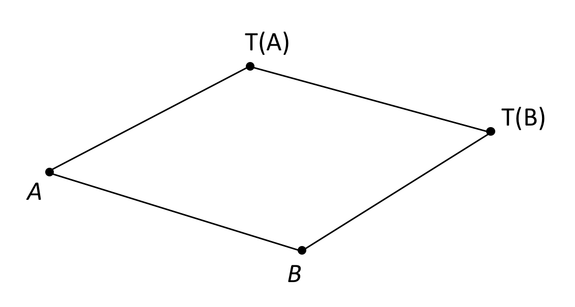
A translation \, T \, of the plane is completely known as soon as the image \, T(A) \, of one point \, A \in P \, is known. Namely, \, T \, is then the one-to-one mapping of \, P \, onto itself such that, if \, B \, is a point of \, P , the four points \, A, B, T(B), T(A) \, form a parallelogram when taken in proper order as shown in Figure 4.1:
If \, T_1 \, and \, T_2 \, are two translations of \, P , their sum \, T_1 + T_2 \, is defined as the composite mapping \, T_1 T_2 : P \rightarrow P , meaning first \, T_2 : P \rightarrow P \, and then \, T_1 : P \rightarrow P .
It is also easy to see how a translation \, T \, is multiplied by a real number \, c . Suppose \, T \, sends the point \, A \, of \, P \, onto the point \, T(A) , that is \, T \, is determined by the vector \, (A, T(A)) . Then \, c T \, is determined by the vector \, c (A, T(A)) . Clearly \, 0T \, is the identity mapping of the plane.
/////// End of quote from Snapper and Troyer.
/////// Quoting Affine geometry at Wikipedia (2018-09-21):
In mathematics, affine geometry is what remains of Euclidean geometry when not using (mathematicians often say “when forgetting”) the metric notions of distance and angle.
As the notion of parallel lines is one of the main properties that is independent of any metric, affine geometry is often considered as the study of parallel lines. Therefore, Playfair’s axiom (given a line L and a point P not on L, there is exactly one line parallel to L that passes through P) is fundamental in affine geometry. Comparisons of figures in affine geometry are made with affine transformations, which are mappings that preserve alignment of points and parallelism of lines.
Affine geometry can be developed in two ways that are essentially equivalent.
• In synthetic geometry, an affine space is a set of points to which is associated a set of lines, which satisfy some axioms (such as Playfair’s axiom).
• Affine geometry can also be developed on the basis of linear algebra. In this context an affine space is a set of points equipped with a set of transformations (that is bijective mappings), the translations, which forms a vector space (over a given field, commonly the real numbers), and such that for any given ordered pair of points there is a unique translation sending the first point to the second; the composition of two translations is their sum in the vector space of the translations.
In more concrete terms, this amounts to having an operation that associates to any ordered pair of points a vector and another operation that allows translation of a point by a vector to give another point; these operations are required to satisfy a number of axioms (notably that two successive translations have the effect of translation by the sum vector).
By choosing any point as “origin”, the points are in one-to-one correspondence with the vectors, but there is no preferred choice for the origin; thus an affine space may be viewed as obtained from its associated vector space by “forgetting” the origin (zero vector).
///////
• Edwin B. Wilson & Gilbert N. Lewis (1912). “The Space-time Manifold of Relativity. The Non-Euclidean Geometry of Mechanics and Electromagnetics“, Proceedings of the American Academy of Arts and Sciences 48:387–507.
• Synthetic Spacetime, a digest of the axioms used, and theorems proved, by Wilson and Lewis. Archived by WebCite
/////// End of quote from Wikipedia
/////// Quoting Snapper and Troyer (1971, p. 6):
Definition 6.1. To say that the additive group of the vector space \, V \, acts on the set \, X \, means that, for every vector \, A \in V \, and every point \, x \in X , there is defined a point \, Ax \in X \, such that:
1. If \, A, B \in V \, and \, x \in X , then \, (A + B)x = A(B(x)) .
2. If \, 0 \, denotes the zero vector, then \, 0 \, x = x \, for all \, x \in X .
3. For every ordered pair \, (x, y) \, of points of \, X ,
there is one and only one vector \, A \in V \, such that \, Ax = y .
The unique vector \, A \, such that \, Ax = y \, will be denoted by \, \overrightarrow{x,y} .
/////// End of quote from Snapper and Troyer.
/////// Quoting Snapper and Troyer (1971, p. 8):
3. A CONCRETE MODEL FOR AFFINE SPACE:
We now look at a model for \, n -dimensional affine space. In fact, the model we are going to describe is often used as the definition of affine space. Let \, V \, be an \, n -dimensional left vector space over a division ring \, k \, . For the set \, X \, , we choose the vectors of \, V \, , that is, \, X = V \, where \, V \, is considered only as a set. The action of the additive group of \, V \, on the set \, V \, is defined as follows:
If \, C \in V \, and \, A \in V , then \, AC = A + C .
Some care must now be taken so that no confusion arises from the fact that we have defined \, X \, to be the set \, V \, .
Exercise: Verify that \, (V, V, k) \, , as defined above, is a model for \, n -dimensional affine space. In other words, prove that the three conditions of Definition 6.1 are satisfied.
The reader has become accustomed in his linear algebra courses to visualize the vector \, A \, of the vector space \, V \, as an arrow starting at \, 0 . When \, V \, is regarded as an affine space, that is, \, X = V , the point \, A \, should be visualized as the end of the arrow.
4. TRANSLATIONS
We now introduce translations into our affine space \, (X, V, k) \, .
Definition 9.1. Let \, A \in V . The functon \, T_A : X \rightarrow X \, defined by \, T_A(x) = A x \, for all \, x \in X \, is called the translation of \, X \, associated with \, A \, .
From our intuitive notion of translations, we certainly expect each translation to be a one-to-one function of \, X \, onto \, X . This fact is indeed true; we shall eventually prove much more about the set of translations.
/////// End of quote from Snapper and Troyer.
In the light of the above, we can model an affine space as a set of points \, p and an additive group of displacements (= translations) \, T_p . To each pair \, (p, T_p) \, corresponds the mapping \, T_p : X \rightarrow X \, with \, T_p(x) = \overrightarrow{x,x + p} .
In affine geometry a vector \, A \, is in fact a displacement vector which defines a rectilinear displacement (= a translation) \, \overrightarrow {x ,A x} \, between the points \, x \, and \, A x .
By choosing any point \, O \, as the origin, the set of translations \, V_O = \{ \, \overrightarrow{O,x} : x \in X \, \} \, forms a vector space, and we have for each pair of points \, x, y \in X \, :
\, \overrightarrow{O,x} + \overrightarrow{O,y} = \overrightarrow{O,x+y} ,
\, \overrightarrow{O,y} = \overrightarrow{O,x} + \overrightarrow{x,y} = \overrightarrow{O,x} + \overrightarrow{O,y-x} ,
\, \overrightarrow{x,y} = \overrightarrow{O,y} - \overrightarrow{O,x} = \overrightarrow{O,y-x} .
AFFINE SUBSPACES
/////// Quoting Snapper and Troyer (1971, p. 11):
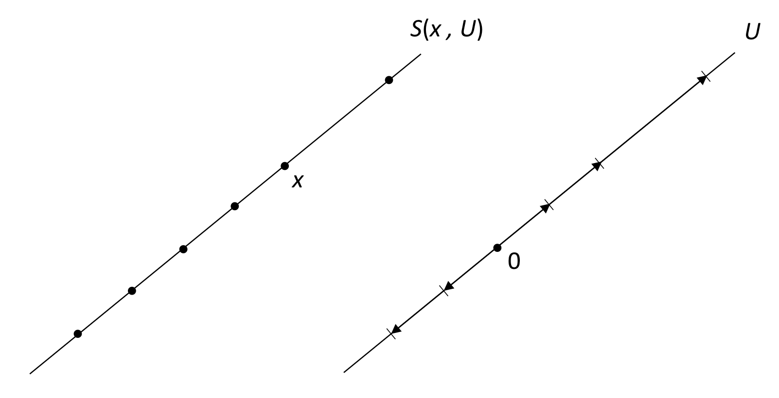
In our study of the \, n -dimensional affine space \, (X, V, k) \, we must say what is meant by lines, planes and, more generally, by the affine subspaces of \, X . An affine subspace \, S(x, U) \, of \, X \, is determined by a point \, x \in X \, and a linear subspace \, U \, of \, V .
Definition 11.1. The affine subspace \, S(x, U) \, of \, X \, consists of the points \, A x \,
where \, A \, is an arbitrary vector of \, U . In short,
\, S(x, U) = \{ Ax \, | \, A \in U \} .
The dimension of the linear subspace \, U \, of \, V \, is also called the dimension of the affine subspace \, S(x, U) \, of \, X . Affine subspaces of dimension one are called lines while those of dimension two are called planes. The affine subspaces of dimension \, n-1 \, are called hyperplanes.
Let us say a few words about the pictures we associate with the affine space \, X \, and its affine subspaces when the dimension of \, X \, is two and three. For dimension two, we picture \, X \, as a physical plane of points with no special points singled out. The sets \, V \, and \, X \, have nothing in common and we picture the elements of \, V \, as arrows beginning at the origin \, 0 . If \, x \in X \, and \, A \in V , we picture the result of the action of \, A \, on \, x \, as in Figure 11.1:

Continuing with dimension two, we suppose that \, U \, is a one-dimensional linear subspace of \, V \, and that \, x \in X . We picture \, U \, and \, S(x, U) \, as in Figure 12.1:
Similarly, if the dimension of \, X \, is three, we visualize \, X \, as the space which surrounds us. If \, U \, is a two-dimensional linear subspace of \, V \, and \, x \in X , we picture \, U \, and the plane \, S(x, U) \, as in Figure 12.2:

Even if \, \textnormal {dim} \, X > 3 , one should force oneself to visualize. Then \, X \, is viewed as a very roomy three-space in which two planes may possibly have only a point in common ( \, \textnormal {dim} \, X = 4 \, ) which cannot happen when \, n = 3 . Also, \, V \, is viewed as an equally roomy bundle of arrows, all starting at the origin \, 0 .
One-dimensional linear subspaces of \, V \, are viewed as lines through \, 0 \, and two-dimensional linear subspaces of \, V \, are viewed as planes through \, 0 . Lines and planes of \, X \, are again viewed as ordinary physical lines and planes. As shown in the following exercise, the affine subspace \, S(x, U) \, must pass through the point \, x .
Exercise 12.3: Prove that \, x \in S(x, U) .
Suppose we are given a subset \, S \, of \, X \, and that we are told there is a point \, x \in X \, and a linear subspace \, U \, of \, V \, such that \, S \, is the affine subspace \, S(x, U) \, of \, X . Can we recover \, U \, by just knowing the pointset \, S \, ?
The answer is yes, as is seen from Proposition 13.1 where the vectors of \, U \, are described intrinsically in therms of the points of \, S . Recall that, if \, x, y \in X, \overrightarrow{x,y} \, denotes the unique vector \, A \in V \, such that \, A x = y .
Proposition 13.1. Let \, S = S(x, U) \, be the affine subspace determined by the point \, x \, and the linear subspace \, U . Then \, U = \{ \overrightarrow {y,z} \, | \, y, z \in S \, \} . Consequently, \, U \, is uniquely determines by \, S(x, U) .
Proof: Let \, A \in U . Then \, x \in S \, (Exercise 12.3) and, by definition of \, S , \, y = A x \in S . Consequently, \, A = \overrightarrow {x,y} \, which shows that \, U \subset \{ \overrightarrow {y,z} \, | \, y, z \in S \, \} . Conversely, let \, y, z \in S \} . Then there exists vectors \, A, B \in U \, such that \, y = A x \, and \, z = B x .
Figure 13.1 below illustrates the situation when \, S \, is a plane.
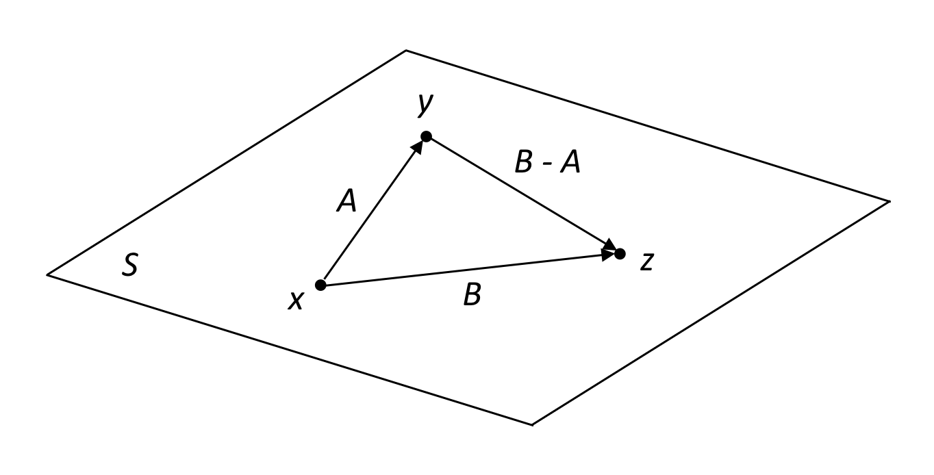
Now, \, y = A x \iff x = (-A) y ;
thus \, z = B x \iff z = B (-A) y = (B - A) y .
Consequently, \, B - A = \overrightarrow{y,z} \, and, since \, B - A \in U, \overrightarrow{y,z} \in U .
This proves that \, U \supset \{ \overrightarrow {y,z} \, | \, y, z \in S \} . Done.
Of course, the pointset \, S(x, U) \, could not possibly determine the point \, x \, uniquely unless \, \textnormal{dim} \, U = 0 . All points of \, S(x, U) \, play the same role!
We now say precisely when two affine subspaces \, S(x, U) \, and \, S(y, W) \, are equal.
Proposition 14.1. Let \, x, y \, be points of \, X \, and \, U, W \, linear subspaces of \, V .
Then \, S(x, U) = S(y, W) \, if and only if \, U = W \, and \, S(x, U) \cap S(y, W) \not = \emptyset .
Proof: If \, S(x, U) = S(y, W) , then \, U = W \, by Proposition 13.1 while both \, x \, and \, y \, belong to \, S(x, U) \cap S(y, W) . Conversely, suppose that \, U = W \, and that \, z \in S(x, U) \cap S(y, U) . We shall prove that \, S(x, U) = S(y, W) \, by showing that both of these spaces are equal to \, S(z, U) .
It is sufficient to show that \, S(x, U) = S(z, U) , the proof that \, S(y, U) = S(z, U) \, being the same. Since \, z \in S(x, U), \, z = A x \, for \, A \in U . If \, B \in U , \, B z = B(A(x)) = (B+A)x \in S(x, U) \, since \, B + A \in U . This shows that \, S(z, U) \subset S(x, U) . For the inverse conclusion, we use the fact that \, x = (-A) z \in S(z, U) . Done.
Definition 14.1: The linear subspace \, U \, of \, V \, is called the direction space of \, S(x, U) .
The dimension of \, S(x, U) \, is, therefore, the dimension of its direction space \, U . Clearly the direction space of \, X \, is \, V .
The term “affine subspace” will now be justified by showing that an affine subspace is an affine space in its own right. For convenience we often write \, S \, for \, S(x, U) \, when there is no danger of confusion.
Proposition 14.2: Let \, S = S(x, U) \, be a \, d -dimensional affine subspace of \, X . Then the triple \, (S, U, k) , together with the action inherited from the affine space \, (X, V, k) , is a \, d -dimensional affine space.
Proof: Let \, A \in U \, and \, y \in S . According to Definition 6.1, we must first show that \, A y \in S . However, \, y = B x \, for \, B \in U \, and hence \, Ay = A(Bx) = (A+B)x \in S \, since \, A + B \in U . The action of \, U \, on \, S \, immediately inherits Properties 1 and 2 of Definition 6.1 from the action of \, V \, on \, X . There remains to be shown only that, if \, y, z \in S , there exists one and only one vector \, A \in U \, such that \, A y = z . The vector \, A = \overrightarrow{y,z} \, belongs to \, U \, (Proposition 13.1) and \, A y = z . Moreover, \, A \, is the only vector in all of \, V \, such that \, A y = z . Done.
Many questions arise. Is the intersection of two affine subspaces an affine subspace? When are two affine subspaces parallel? How does one assign a coordinate system to an affine subspace? Questions of this nature will now be considered.
/////// End of quote from Snapper and Troyer.
//// MUST SET THE CONTEXT HERE: e.g., introduce \, V_o \,
Two points \, a \, and \, b \, in \, X \, span an affine subspace of dimension one, which represents a line. In \, V_o \, this line can be parametrised as
\, \{ \lambda \, \overrightarrow{o,a} + (1-\lambda) \, \overrightarrow{o,b} : \lambda \in \mathbf {R} \} .
The difference between two displacement vectors is called a direction vector (or a Euclidean vector). The direction vector \, a - b \, spans a linear subspace that is parallel to the affine subspace spanned by the displacement vectors \, a \, and \, b \, .

This picture shows the linear space probe used to explore the rank-nullity theorem of a linear transformation.
In the probe, the red centre line and the grey centre plane form linear subspaces, while the yellow lines and the light-blue planes form affine subspaces. Hence, from the relationship between of affine geometry and Euclidean geometry (discussed above) we can conclude that:
• if the tips of two displacement vectors lie on the same yellow line,
then the direction vector of their difference lies in the red centre line.
• if the tips of two or more displacement vectors lie on the same light-blue plane,
then the direction vectors of their pairwise differences lie in the grey centre plane.
Geometrically, the take-away lesson from this discussion is that:
• A displacement vector represents a change of position called a translation.
• A direction vector represents a change of direction. Such a change of direction has both a direction and a magnitude. The magnitude of a direction vector corresponds to the magnitude of the directional change that it represents.
• The difference between two displacement vectors is a direction vector.
• The affine subspace spanned by a finite number of displacement vectors is parallel to the linear subspace spanned by the direction vectors of their pairwise differences.