This is a sub-page of our page on Projective Geometry
///////
The sub-pages of this page are:
///////
The interactive simulations on this page can be navigated with the Free Viewer
of the Graphing Calculator.
///////
Related sources of information:
• Projective determination of a metric
• Cayley-Klein Metric
• Laguerre’s angle formula
• Laguerre Planes
• Trilinear Polar
///////
Representation:
[ \, [ \, a_{bsolute} \,]_{L_{ocus}} \, ]_{N_{on}D_{egenerated}G_{eometry}} = \left< \, p_{oint} c_{onic} \, \right>_{N_{on}D_{egenerated}G_{eometry}}
Representation:
[ \, [ \, a_{bsolute} \,]_{E_{nvelope}} \, ]_{N_{on}D_{egenerated}G_{eometry}} = \left< \, l_{ine} c_{onic} \, \right>_{N_{on}D_{egenerated}G_{eometry}}
IMPORTANT: The \, c_{onic} \, appearing in the locus- and the envelope representations of the \, a_{bsolute} \, of a non-degenerated geometry is THE SAME \, c_{onic} \, . This is why there is complete duality between distance-geometry and angle-geometry in any non-degenerated geometry.
When the geometry degenerates, the absolute conic degenerates differently as a locus (= point-conic) and as an envelope (= line-conic). This difference breaks up the complete duality between distance and angle that is characteristic of non-degenerate geometries.
Representation: [ \, [ \, a_{bsolute} \,]_{L_{ocus}} \, ]_{E_{uclidean}G_{eometry}} = \left< \, d_{ouble} l_{ine} \, \right>_{E_{uclidean}G_{eometry}}
Representation: [ \, [ \, a_{bsolute} \,]_{E_{nvelope}} \, ]_{E_{uclidean}G_{eometry}} = \left< \, t_{wo} l_{ine} p_{encils} \, \right>_{E_{uclidean}G_{eometry}}
When the absolute conic is real, the geometry is called hyperbolic and when the absolute conic is imaginary, the geometry is called elliptic. When the absolute conic degenerates, into a double line, the geometry is called parabolic.
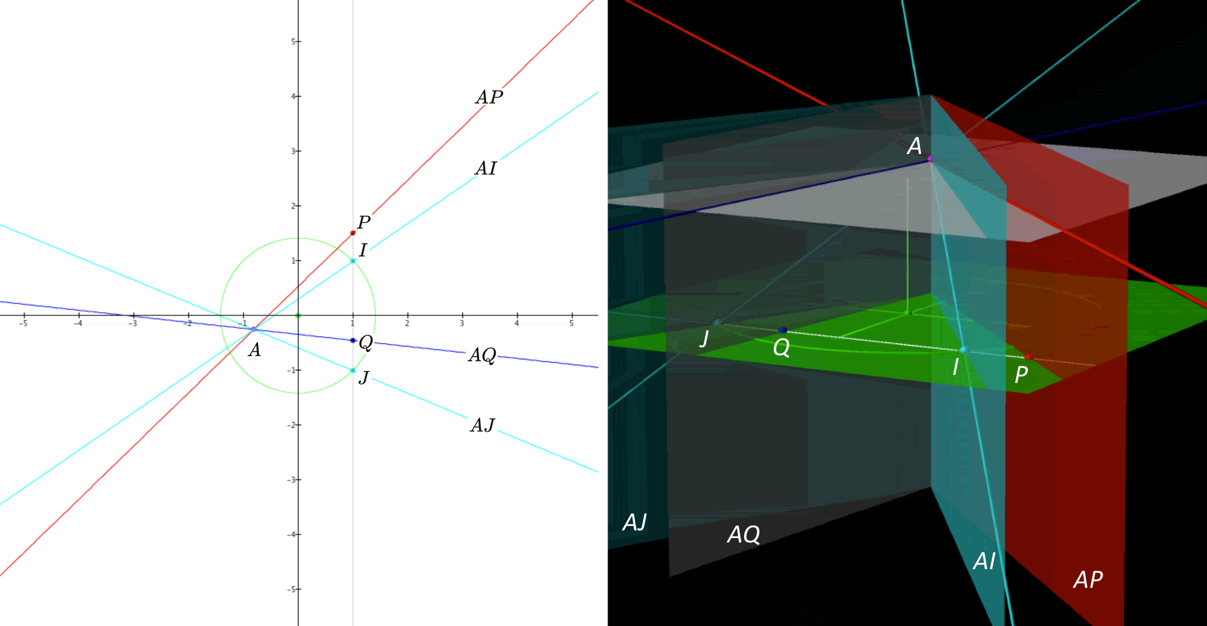
Euclidean geometry has a parabolic distance geometry and an elliptic angle geometry. The euclidean absolute point-locus is the line at infinity ( \, z = 0 \, ) taken twice, and the euclidean absolute envelope are the two pencils of lines on the two conjugate complex points \; I = (1 : i : 0) \; and \, J = (1 : -i : 0) \, . They are called the circular points, since all euclidean circles pass through them.
///////
Representation: [ \, \infty \, ]_{E_{uclidean}G_{eometry}} = \left< \, \nexists \, \right>_{E_{uclidean}G_{eometry}} \,
Representation: [ \, \infty \, ]_{P_{rojective}G_{eometry}} = \left< \, l_{ine} \, \right>_{P_{rojective}G_{eometry}} \,
Representation: [ \, \infty \, ]_{P_{rojective}M_{etrics}} = \left< \, c_{onic} \, \right>_{P_{rojective}M_{etrics}} \,
Representation: [ \, \infty \, ]_{\mathbb{P}^2 M_{etrics}} = \left< \, c_{onic} \, \right>_{\mathbb{P}^2 M_{etrics}} \,
Representation: [ \, \infty \, ]_{\mathbb{P}^3 M_{etrics}} = \left< \, q_{uadric} \, \right>_{\mathbb{P}^3 M_{etrics}} \,
///////
Below we make the following summation convention (due to Einstein):
\, {\omega}^i x_i \stackrel {\mathrm{def}}{=}{\sum\limits_{1 \le k \le n+1}^{ \text {} } {\omega}^k x_k} \, .
///////
Let \, X \, and \, \omega \, denote a point and a hyperplane in \, P^3 \, , and let
\,{\lbrack \, X \, \rbrack}_{C.T.U} = ( x_1 : x_2 : x_3 : x_4 ) = (x : y : z : t) \, , and
\,{\lbrack \, \omega \, \rbrack}_{c.t.u} = ( {\omega}^1 : {\omega}^2 : {\omega}^3 : {\omega}^4 ) = (u : v : w : p) \,
denote their respective coordinates in two dually unified systems.
Then the point \, X \, and the plane \, \omega \, are incident if and only if
\, {\omega}^i x_i = 0 \, .
///////
The Poncelét-Gergonne (bilinear form) duality can be expressed as
\, ux+vy+wz+pt=0 \,
or, using index notation:
\, {\omega}^1 x_1+{\omega}^2 x_2+{\omega}^3 x_3 + {\omega}^4 x_4 = 0 \, .
A centrally symmetric quadratic form in point coordinates can be expressed as:
\, \dfrac{x^2}{a}+\dfrac{y^2}{b}+\dfrac{z^2}{c} = t^2 \,
The same quadratic form in plane coordinates:
\, au^2+bv^2+cw^2 = p^2 \,
///////
\, \begin{matrix} {\begin{matrix} \\ \text{Point coordinates:} \\ \\ {x^2/a+y^2/b+z^2/c = t^2} \\ \\ {x^2+y^2+z^2-\frac{1}{\epsilon}t^2 = 0} \\ \\ \begin{matrix} {\epsilon \rightarrow 0 \text{ leads to a logical collapse:}} \\ \\ {x^2+y^2+z^2 = 0} \\ {t^2 = 0} \end{matrix} \end{matrix}} & {\; \; \; \; \; \; \; \; \; \;} & {\begin{matrix} \text{Plane coordinates:} \\ \\ {au^2+bv^2+cw^2 = p^2} \\ \\ {u^2+v^2+w^2-{\epsilon}p^2 = 0} \\ \\ {\epsilon \rightarrow 0 \text{ is unproblematic:}} \\ \\ {u^2+v^2+w^2 = 0} \end{matrix}} \end{matrix} \,
///////
Distance metric:
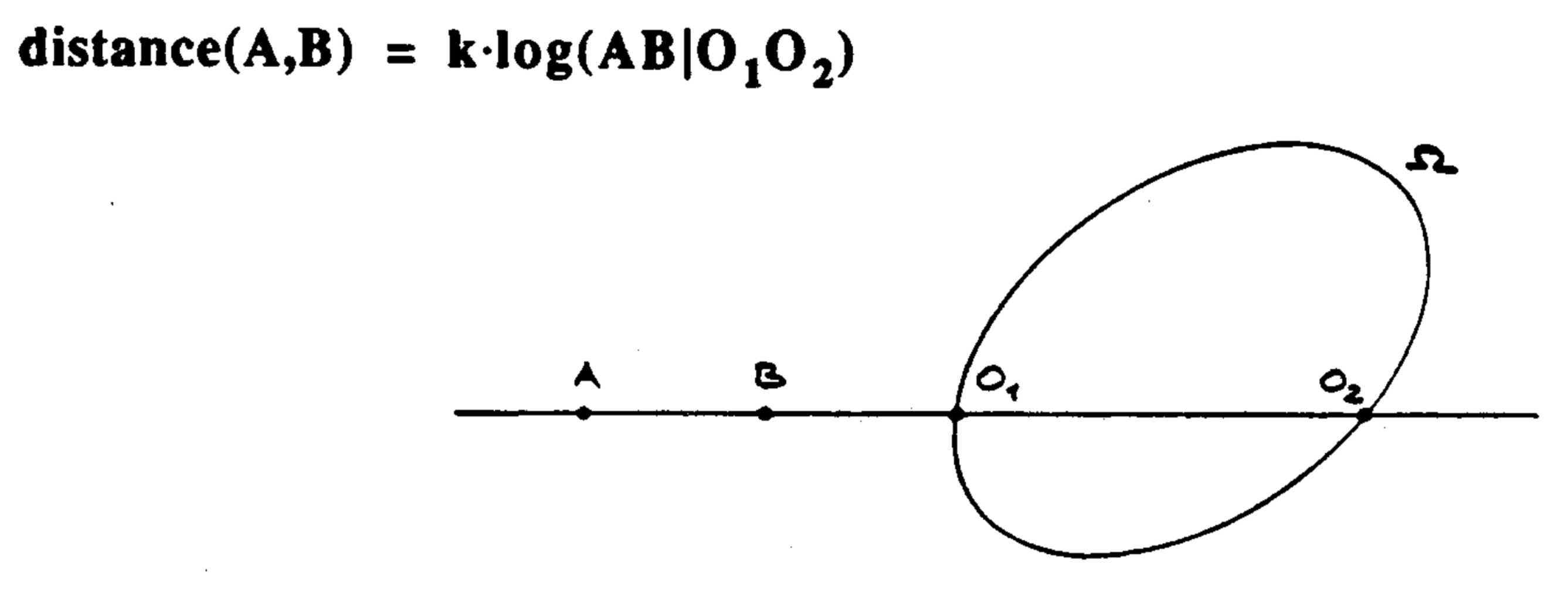
\, d_{istance}(A,B) \stackrel {\mathrm{def}}{=} k \log(AB|O_1 O_2) .
///////
Angle metric:
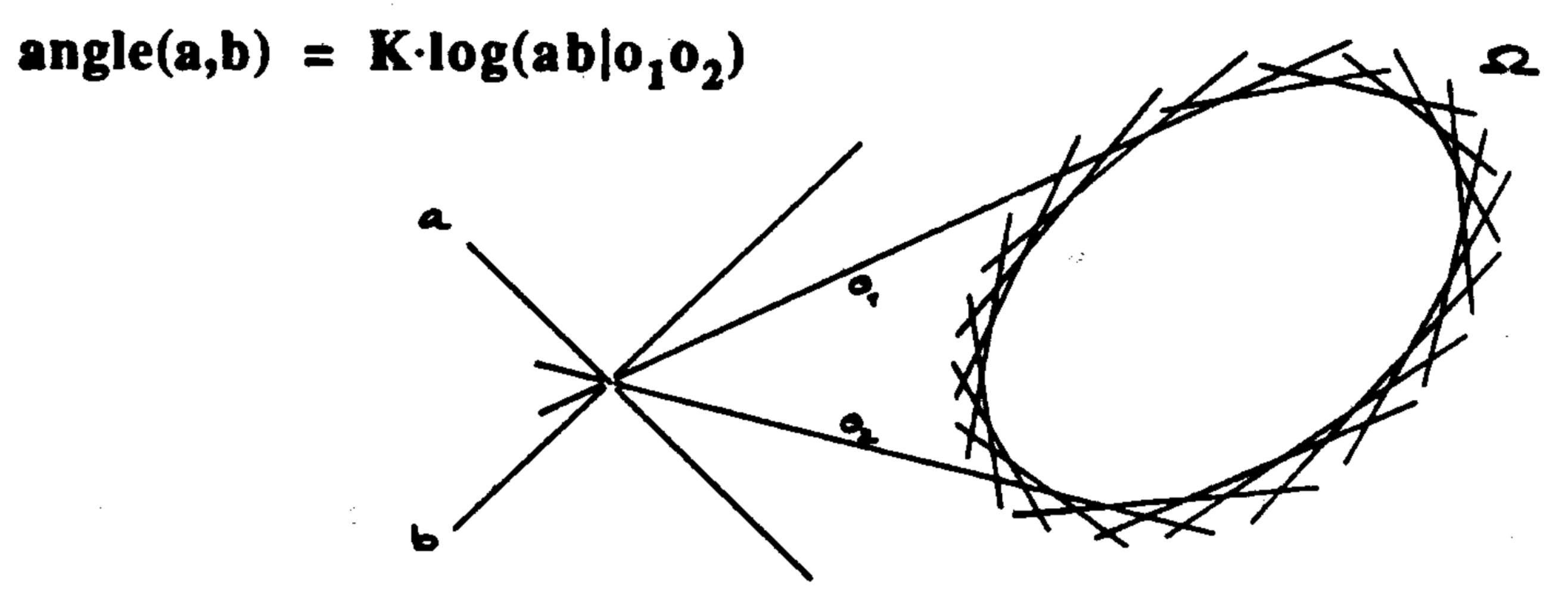
\, a_{ngle}(a,b) \stackrel {\mathrm{def}}{=} k \log(ab|o_1 o_2) .
///////
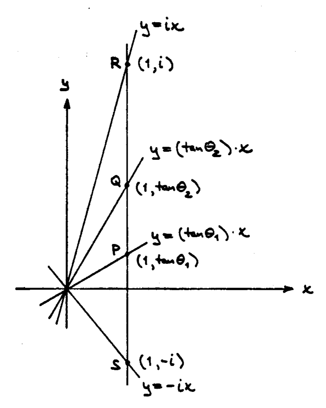
Laguerre’s angle formula:
Laguerre’s angle formula(diagram):
///////
///////
Laguerre’s angle formula – computation:
\, (PQ|IJ) = \dfrac{IP/IQ}{JP/JQ} = \dfrac{\dfrac{i-tan{\theta}_1}{i-tan{\theta}_2}}{\dfrac{-i-tan{\theta}_1}{-i-tan{\theta}_2}} = \,
\, = \dfrac{(i cos{\theta}_1 - sin{\theta}_1)(-i cos{\theta}_2 - sin{\theta}_2)}{(-i cos{\theta}_1 - sin{\theta}_1)(i cos{\theta}_2 - sin{\theta}_2)} = \,
\, = \dfrac{(cos{\theta}_1 + i sin{\theta}_1)(cos{\theta}_2 - i sin{\theta}_2)}{( cos{\theta}_1 - i sin{\theta}_1)(cos{\theta}_2 + i sin{\theta}_2)} = \dfrac{e^{i{{\theta}_1}} e^{-i{{\theta}_2}}}{e^{-i{{\theta}_1}} e^{i{{\theta}_2}}} = \dfrac{e^{i({{\theta}_1 - {\theta}_2})}}{e^{-i({{\theta}_1 - {\theta}_2})}} = ,
\, = e^{2 i({{\theta}_1 - {\theta}_2})} .
We see that if we choose the constant \, k = \frac{1}{2i} \, this formula is indeed expressing the familiar euclidean angle. This calculation was discovered by the sixteen year old Edmund Laguerre in 1853, and it is referred to as Laguerre’s angle formula:
\, \frac{1}{2i} \log(PQ|IJ) = {{\theta}_1 - {\theta}_2} .