This page is a sub-page of our page on Projective Metrics.
///////
Related KMR-pages:
• Projective geometry
• Metric geometry
• Projective metrics
• Non-Euclidean geometry
• Hyperbolic geometry
• Elliptic geometry
///////
Books:
• Felix Klein (1926), Vorlesungen über Nichteuklidische Geometrie,
Verlag von Julius Springer in Berlin, (1928).
• Jürgen Richter-Gebert (2011), Perspectives on Projective Geometry – A Guided Tour Through Real and Complex Geometry, Springer, ISBN 978-3-642-17285-4.
• D.M.Y. Sommerville (1914), The Elements of Non-Euclidean Geometry, Dover (1958, 2005).
• Henry Parker Manning (1901), Introductory Non-Euclidean Geometry, Dover (1963, 2005).
• H.S.M. Coxeter (1947 (1942)), Non-Euclidean Geometry.
• John Stillwell (2016), Elements of Mathematics – From Euclid to Gödel,
Princeton University Press, ISBN 978-0-691-17854-7.
• John Stillwell (1999, (1989)), Mathematics and Its History, Springer, ISBN 0-387-96981-0.
• Jeremy Gray (2007), Worlds Out of Nothing – A Course in the History of Geometry in the 19th Century, Springer, ISBN 1-84628-632-8.
///////
The interactive simulations on this page can be navigated with the Free Viewer
of the Graphing Calculator.
///////
/////// Quoting Sommerville (1914/2005, pp. 155-156):
4. Euclidean geometry
Euclidean geometry is a limiting case, where the space-constant \, k \to \infty \, . The coordinates of a point become the usual rectangular coordinates \, x\, and \, y \, with \, z = 1 \, .
The equation of the absolute becomes in point-coordinates \, z^2 = 0 \, , and in line-coordinates \, \xi^2 + \eta^2 = 0, \, , i.e. the absolute degenerates as a locus to a straight line counted twice – the straight line at infinity, and as an envelope to two imaginary pencils of lines \, \xi + i \eta = 0 \, and \, \xi - i \eta = 0 \, , whose vertices lie on the line at infinity since the line-coordinates of their join are \, \xi = 0, \eta = 0, \zeta = \zeta, \, and its equation is therefore \, z = 0 \, .
The equations of the lines of these imaginary pencils are of the forms
\, x + i y + c z = 0, x - i y + c z = 0 \, .
The formula for the distance between two points,
\, \cos \dfrac{r}{k} = \dfrac{xx'+yy'+k^2zz'}{\sqrt{x^2+y^2+k^2z^2} \sqrt{x'^2+y'^2+k^2z'^2}} \, ,
becomes
\, 1 - \dfrac{1}{2} \, \dfrac{r^2}{k^2} = (xx'+yy'+k^2) \, \dfrac{1}{k^2} \, (1 - \dfrac{1}{2} \, \dfrac{x^2 + y^2}{k^2}) \, (1 - \dfrac{1}{2} \, \dfrac{x'^2 + y'^2}{k^2}) = \,
\, = (1 + \dfrac{xx' + yy'}{k^2}) \, (1 - \dfrac{1}{2} \, \dfrac{x^2 + y^2 + x'^2 + y'^2}{k^2}) = \,
\, = 1 - \dfrac{1}{2} \, \dfrac{(x - x')^2 + (y - y')^2}{k^2} \, ,
or
\, r^2 = (x-x')^2 + (y - y')^2 \, .
/////// End of quote from Sommerville (1914/2005)
Traversing the unit hyperbola
both as a locus and as an envelope:
The interactive simulation that created this movie.
///////
Approaching the euclidean absolute locus at infinity
through the hyperbolic absolute locus:
The interactive simulation that created this movie.
///////
Traversing the hyperbolic absolute locus
close to euclidean infinity:
The interactive simulation that created this movie.
///////
Two finite double-fixpoint harmonic yardsticks:
The interactive simulation that created this movie.
///////
Two similarity-related euclidean distance yardsticks
result as a limit when the double-fixpoint moves out towards infinity:
The interactive simulation that created this movie.
Angle geometry:
Approaching the euclidean absolute envelope at infinity
through the hyperbolic absolute envelope:
The interactive simulation that created this movie.
///////
Traversing the hyperbolic absolute envelope
close to euclidean infinity:
The interactive simulation that created this movie.
///////
Approaching the euclidean absolute envelope at infinity
through the elliptic absolute envelope:
The interactive simulation that created this movie.
///////
Traversing the elliptic absolute envelope
close to euclidean infinity:
The interactive simulation that created this movie.
///////
/////// Quoting Sommerville (1914/2005, pp. 156):
5. The circular points
The equation of a circle becomes of the general form
\, x^2 + y^2 + z ( ax + by + cz ) = 0 \, ,
and this represents a conic passing through the points of intersection of the line \, z = 0 \, with the pair of imaginary lines \, x + i y = 0 \, and \, x - i y = 0 \, , i.e. every circle passes through the vertices of the imaginary pencils. For this reason these two points are called the circular points. This property of the circle is the equivalent of the property that it has double contact with the absolute. (Chap.IV.§16.)
/////// End of quote from Sommerville (1914/2005)
Visualizing the circular points: \; I = (1 : i : 0) \, and \, J = (1 : -i : 0) \, :
Approaching the euclidean absolute envelope
through an elliptic absolute envelope:
The interactive simulation that created this movie.
///////
Approaching the euclidean absolute envelope
through a hyperbolic absolute envelope:
The interactive simulation that created this movie.
/////// The elliptic approach to the euclidean absolute envelope:
Laguerre (elliptic new) (lettered) (s = 5.5).png:
An elliptic absolute envelope (s = 5.5) having double contact
with the euclidean absolute envelope:
Getting closer to the euclidean absolute envelope:
///////
An elliptic absolute envelope (s = 23.7)
is getting close to the euclidean absolute envelope:
The interactive simulation that created the two movies above (for s = 5.5 respectively s = 23.7).
///////
Reaching the euclidean absolute envelope,
which is the two pencils on the circular points \, I \, and \, J \,
as the limit when s has “become infinite”:
Laguerre (euclidean – dragable point A (lettered):
///////
The euclidean absolute envelope
appears as the limit of the elliptic absolute envelopes
when the parameter s tends to infinity:
The interactive simulation that created this movie.
///////
The euclidean absolute envelope: Moving the point \, A \,
The angle between the lines \, AP \, and \, AQ \, can be computed using Laguerre’s angle formula.
The interactive simulation that created this movie.
///////
Laguerre’s angle formula
(computation):
\, (PQ|IJ) = \dfrac{IP/IQ}{JP/JQ} = \dfrac{\dfrac{i \, - \, \tan{\theta}_1}{i \,- \, \tan{\theta}_2}}{\dfrac{-i \, - \, \tan{\theta}_1}{-i \, - \, \tan{\theta}_2}} = \,
\, = \dfrac{(\, i \, \cos{\theta}_1 \, - \, \sin{\theta}_1 \,) \, ( \, -i \, \cos{\theta}_2 \, - \, \sin{ \theta}_2 \, )}{(\, -i \, \cos{\theta}_1 \, - \, \sin{\theta}_1) \, ( \, i \, \cos{ \theta}_2 \, - \, \sin{\theta}_2 \,)} = \,
\, = \dfrac{(\, \cos{\theta}_1 \, + \, i \, \sin{\theta}_1) \, (\cos{\theta}_2 \, - \, i \, \sin{\theta}_2)}{(\cos{\theta}_1 \, - \, i \, \sin{\theta}_1) \, (\cos{\theta}_2 \, + \, i \, \sin{\theta}_2 \,)} = \,
\, = \dfrac{e^{\, i {{\theta}_1}} \, e^{-i {{\theta}_2}}} {{ e^{-i {{\theta}_1}} \, e^{\, i {\theta}_2}}} = \dfrac{e^{ \, i ({\theta}_1 \, - \, {\theta}_2)}} {e^{-i ({\theta}_1 \, - \, {\theta}_2)}} = e^{\, 2 i ({{ \theta}_1 \, - \, {\theta}_2})} .
We see that if we choose the constant \, k = 1/2i \, this formula is indeed expressing the familiar euclidean angle. This calculation was discovered by the sixteen year old Edmund Laguerre in 1853, and it is referred to as Laguerre’s angle formula:
\, \dfrac{1}{2i} \log \, (PQ|IJ) = {{\theta}_1 - {\theta}_2} .
///////
CHANGING from depicting THE ABSOLUTE as x^2 + y^2 = 2, z^2 = 0,
to depicting it as x^2 + y^2 = 0 , z^2 = 0 \,
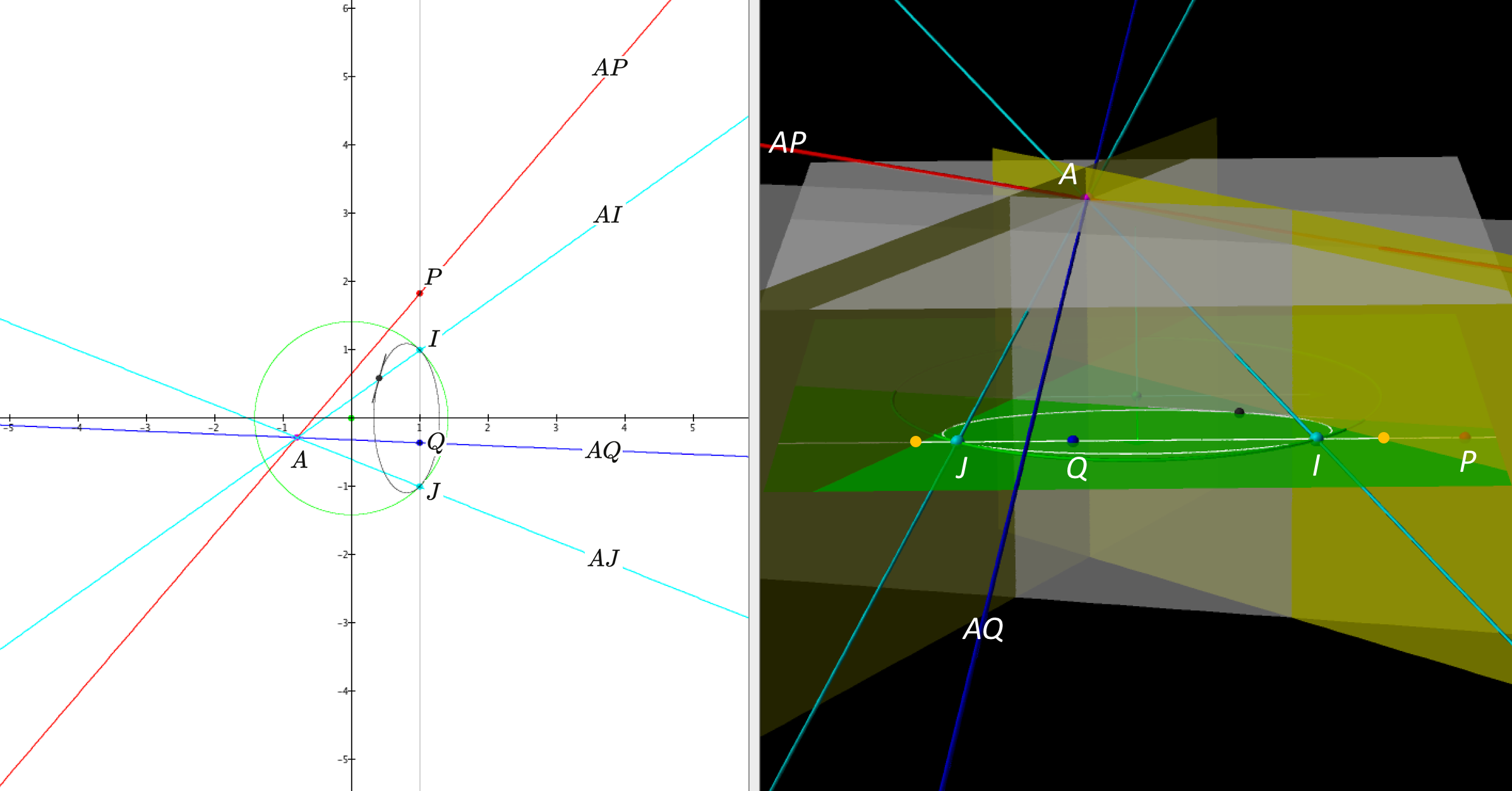
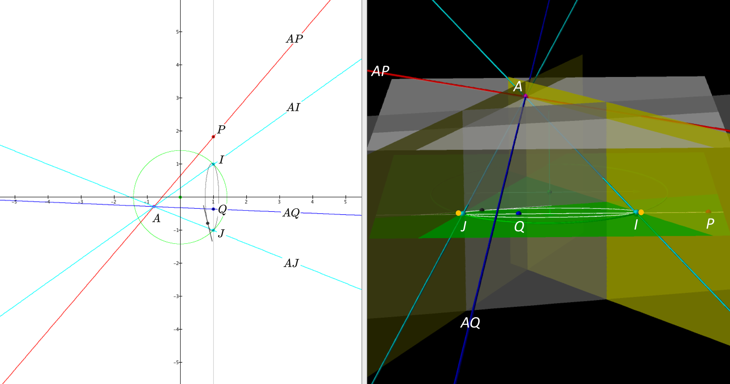
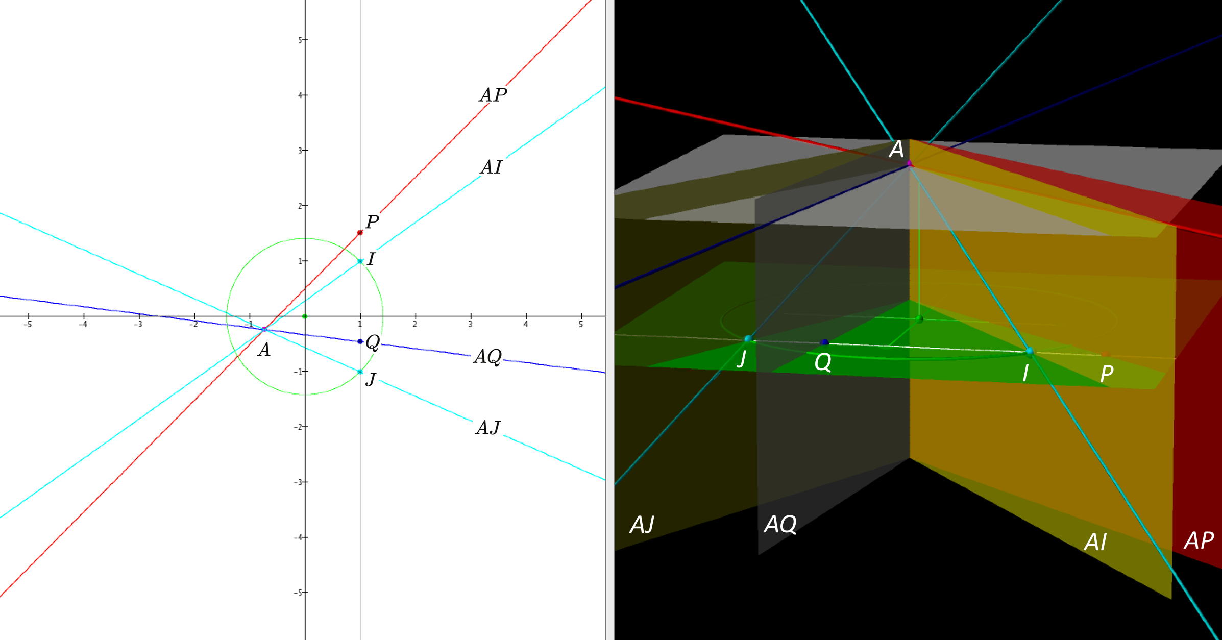
Visualizing the circular points
(with the absolute depicted as \, x^2 + y^2 = 0, z^2 = 0 \, ):
The interactive simulation that created this movie.
/////////////
Distance geometry:
/////// Quoting Richter-Gebert (2011, p. 345 – 346):
Using \, I \, and J \, we can also express distances between two points \, P \, and \, Q \, in Euclidean geometry. This formula is a little bit “tricky,” and we will present it here without a strictly formal proof. First of all, we cannot expect to express the distance purely as a projectively invariant formula only involving \, P, Q, I \, and \, J , since distance is not an invariant of similarity geometry.
The only thing we can hope for is that we obtain a formula that compares the distance between \, P \, and \, Q \, to the distance between two reference points \, A \, and \, B . Thus we will compute a formula for \, |P,Q|/|A,B| \, . If the distance \, |A,B| \, is normalized to be the unit length, we will have a formula for the distance of two arbitrary points. We will finally have an invariant expression in the six points \, A, B, P, Q, I, J .
For two points \, P = (p_1, p_2) \, and \, Q = (q_1, q_2) \, in the Euclidean plane \, {\mathbb R}^2 \, , we usually calculate the distance via the Pythagorean theorem:
\, |P,Q| = \sqrt { {(p_1 - q_1)}^2 + {(p_2 - q_2)}^2 } .
We will first express this formula in terms of determinants and then enlarge this formula to get a projectively invariant expression. Again we assume that \, P \, and \, Q \, have homogeneous coordinates with respect to the standard embedding. Thus we have \, P = {(p_1, p_2, 1)}^T \, and \, Q = {(q_1, q_2, 1)}^T .
We now consider the expression \, \sqrt { [P,Q,I] [P,Q,J] } . Expanding this term, we get
\, \sqrt { \begin{vmatrix} p_1 & q_1 & -i \\ p_2 & q_2 & 1 \\ 1 & 1 & 0 \end{vmatrix} \begin{vmatrix} p_1 & q_1 & i \\ p_2 & q_2 & 1 \\ 1 & 1 & 0 \end{vmatrix} } = \sqrt { ((q_1 - p_1) + i(q_2 - p_2)) \, ((q_1 - p_1) - i(q_2 - p_2)) } = \,
\, = \sqrt { {(p_1 - q_1)}^2 + {(p_2 - q_2)}^2 } = |P,Q| .
This is exactly the desired distance. Unfortunately, the expression
\, \sqrt { [P,Q,I] [P,Q,J] } \,
is not at all a projective invariant. The following expression, however, is:
\, \dfrac { \sqrt {[P,Q,I] [P,Q,J]} [A,I,J] [B,I,J] } { \sqrt {[A,B,I] [A,B,J]} [P,I,J] [Q,I,J] } = |P,Q| .
This expression is indeed a projective invariant (each letter occurs with the same power in numerator and denominator). Furthermore, for the case of the standard embedding and \, |A,B| = 1 \, we get exactly the right distance function (as the following comparison of terms shows):
\, \dfrac { \sqrt {[P,Q,I] [P,Q,J]} [A,I,J] [B,I,J] } { \sqrt {[A,B,I] [A,B,J]} [P,I,J] [Q,I,J] } = |P,Q| .
All in all we get the following result:
Theorem 18.10. The Euclidean distance \, |P,Q| \, between two points \, P \, and \, Q \,
can be calculated by
\, \dfrac { \sqrt {[P,Q,I] [P,Q,J]} [A,I,J] [B,I,J] } { \sqrt {[A,B,I] [A,B,J]} [P,I,J] [Q,I,J] } = |P,Q| ,
if \, |A,B| = 1 \, is a reference length.
/////// End of quote from Richter-Gebert (2011).
///////
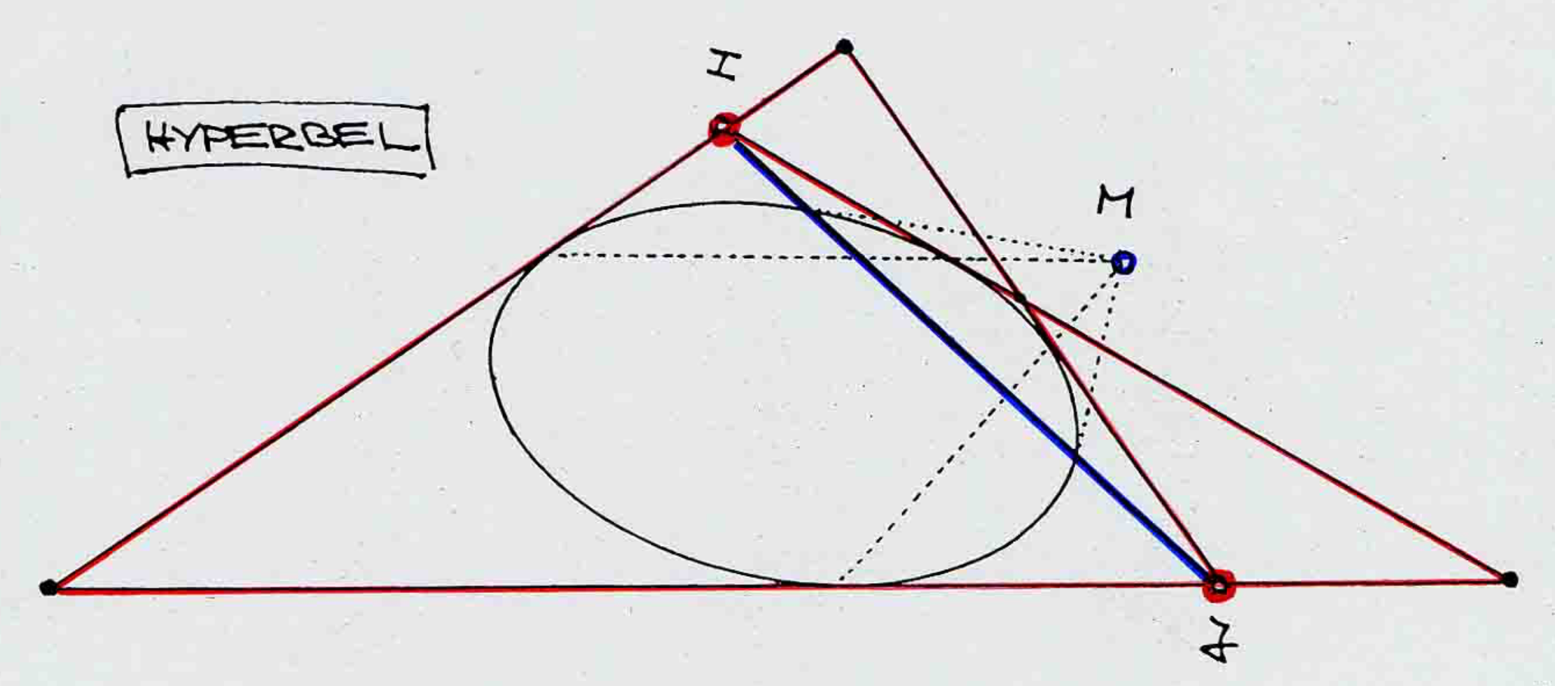
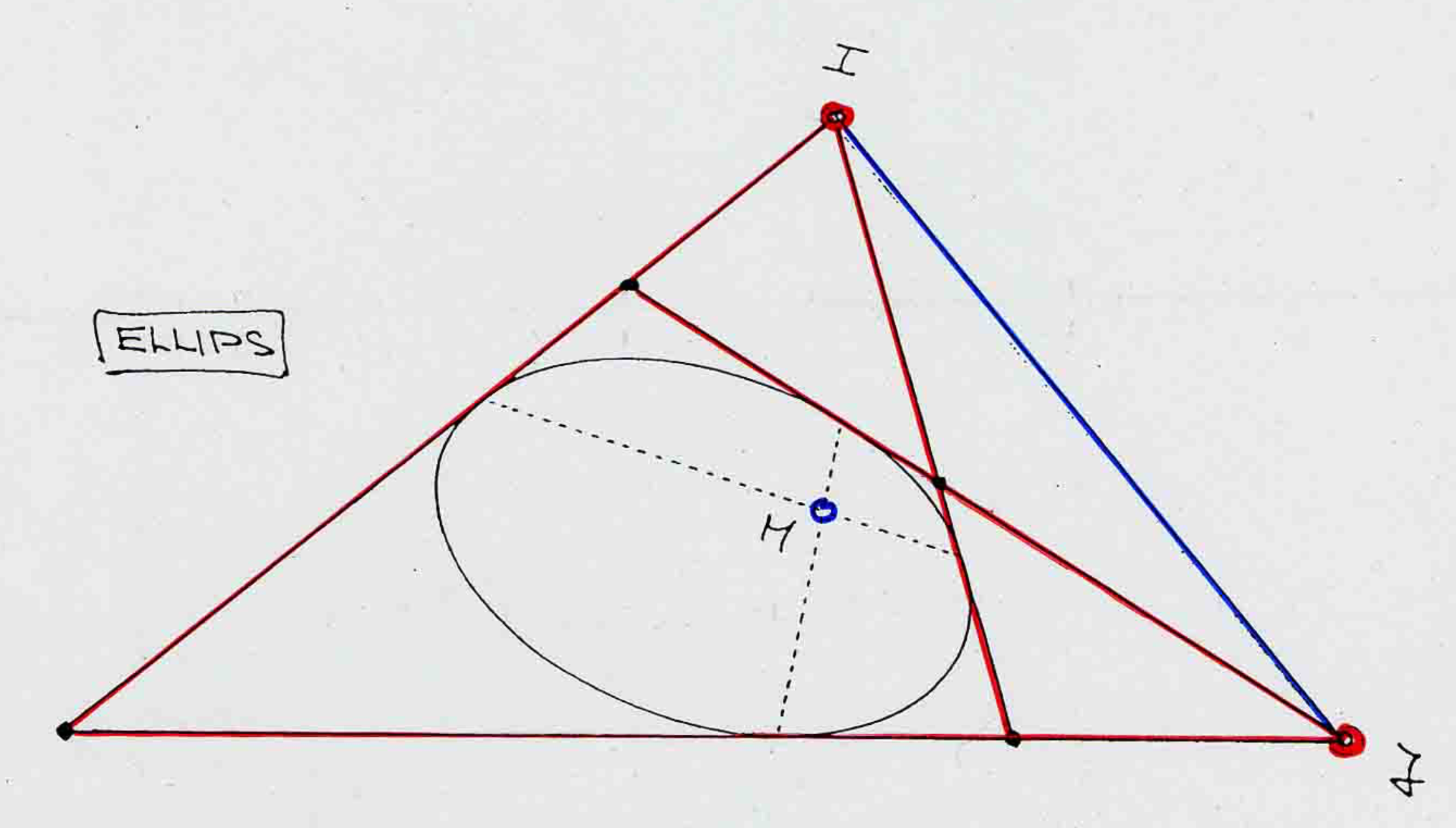
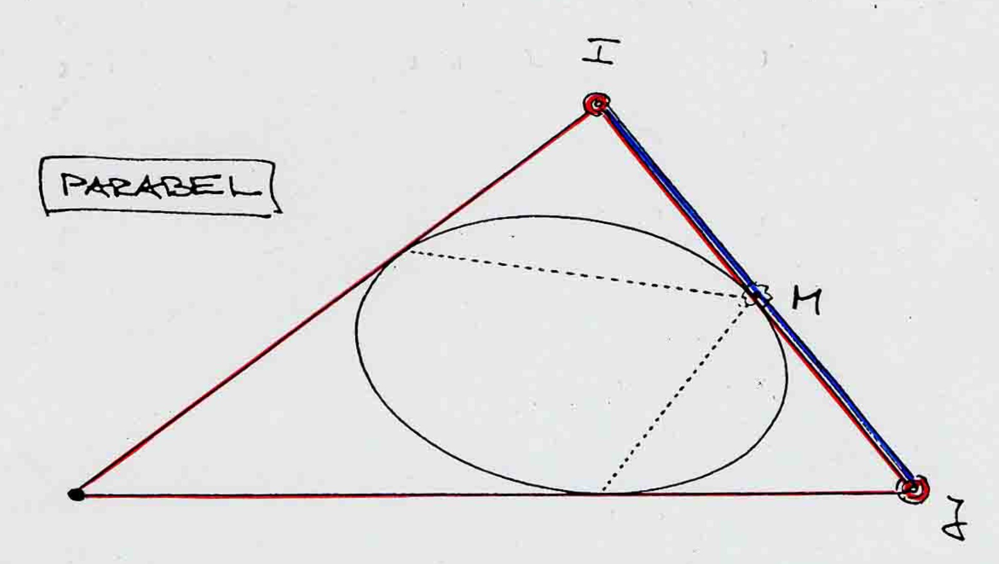
The focal points of a conic depend on the relationship of this conic to the absolute conic:
Ellipse:
Parabola:
Hyperbola: