This page is a sub-page of our page on New Foundations for Classical Mechanics.
///////
Related KMR-pages:
• Chapter 1: Origins of Geometric Algebra
• Chapter 3: Mechanics of a Single Particle
• Chapter 4: Central Forces and Two-Particle Systems
///////
Books:
• René Descartes (1637), La Géometrie
• Hermann Günther Graßmann (1844), Die Lineale Ausdehnungslehre, ein neuer Zweig der Mathematik
• A New Branch Of Mathematics – The Ausdehnungslehre of 1844 and Other Works, translated by Lloyd C. Kannenberg (1995)
• William Kingdon Clifford (1878), Applications of Grassmann’s Extensive Algebra, American Journal of Mathematics Vol. 1, No. 4 (1878), pp. 350-358 (9 pages), Published by: The Johns Hopkins University Press
• David Hestenes (1993, (1986)), New Foundations for Classical Mechanics
• Zwikker (1963)
///////
Other relevant sources of information:
///////
/////// Quoting Hestenes: New Foundations for Classical Mechanics (Chapter 2):
Chapter 2: Developments in Geometric Algebra
///////
Table Of Content
2-1. Basic Identities and Definitions
2-2. The Algebra of a Euclidean Plane [Empty]
2-3. The Algebra of Euclidean 3-Space
2-4. Directions, Projections and Angles
2-5.
2-6. Analytic Geometry
///////
In Chapter 1 we developed geometric algebra as a symbolic system for representing the basic geometrical concepts of direction, magnitude, orientation and dimension. In this chapter we continue the development of geometric algebra into a full-blown mathematical language. The basic grammar of this language is completely specified by the axioms set down at the end of Chapter 1. But there is more to a language than its grammar!
To develop geometric algebra to the point where we can express and explore the ideas of mechanics with fluency, in this chapter we introduce auxiliary concepts and definitions, derive useful algebraic relations, describe simple curves and surfaces with algebraic equations, and formulate the fundamentals of differentiation and integration with respect to scalar variables. Further mathematical developments are given in Chapter 5.
2-1. Basic Identities and Definitions
In Chapter 1 we were led to the geometric product for vectors by combining inner and outer products according to the equation
\, \bold a \, \bold b = \bold a \cdot \bold b + \bold a \wedge \bold b. \;\;\;\;\;\;\;\;\;\;\;\;\;\;\;\;\;\;\;\;\;\;\;\;\;\;\;\;\;\;\;\;\;\;\;\;\;\;\;\;\;\;\;\;\;\;\;\;\;\;\;\;\;\;\;\;\;\;\;\;\;\;\;\;\;\;\; (1.1)
Then we reversed the procedure, defining the inner and outer products in terms of the geometric product by the equations
\, \bold a \cdot \bold b = \frac{1}{2} \, (\bold a \, \bold b + \bold b \, \bold a) \;\;\;\;\;\;\;\;\;\;\;\;\;\;\;\;\;\;\;\;\;\;\;\;\;\;\;\;\;\;\;\;\;\;\;\;\;\;\;\;\;\;\;\;\;\;\;\;\;\;\;\;\;\;\;\;\;\;\;\;\;\;\;\;\;\; (1.2)
\, \bold a \wedge \bold b = \frac{1}{2} \, (\bold a \, \bold b - \bold b \, \bold a) \;\;\;\;\;\;\;\;\;\;\;\;\;\;\;\;\;\;\;\;\;\;\;\;\;\;\;\;\;\;\;\;\;\;\;\;\;\;\;\;\;\;\;\;\;\;\;\;\;\;\;\;\;\;\;\;\;\;\;\;\;\;\;\;\, (1.3)
This did more than reduce two different kinds of multiplication to one. It made possible the formulation of a simple axiom system from which an unlimited number of geometrical relations can be deduced by algebraic manipulation. In this section we aim to improve our skills at carrying out such deductions and establish some widely useful results.
The inner and outer product appear frequently in applications, because they have straightforward geometrical interpretations, as we saw in Chapter 1. For this reason, it is often desirable to operate directly with inner and outer products, even though we regard the geometric product as more fundamental. To make this possible, we need a system of algebraic identities relating inner and outer products. We derive these identities, of course, by using the geometric product and the axioms of geometric algebra set down in Section 1-7.
The different products are most easily related by the equation
\, \bold a \, {\bold A}_r = \bold a \cdot {\bold A}_r + \bold a \wedge {\bold A}_r, \;\;\;\;\;\;\;\;\;\;\;\;\;\;\;\;\;\;\;\;\;\;\;\;\;\;\;\;\;\;\;\;\;\;\;\;\;\;\;\;\;\;\;\;\;\;\;\;\;\;\;\;\;\;\;\;\;\;\;\;\, (1.4)
which generalizes (1.1) to apply to any \, r -blade \, {\bold A}_r , and therefor to any \, r -vector (= sum of \, r -blades) with grade \, r > 0 . Recall that the corresponding definition of inner and outer products are given by
\, \bold a \cdot {\bold A}_r = \frac{1}{2} ( \bold a \, {\bold A}_r - (-1)^r \, {\bold A}_r \, \bold a ) = (-1)^{r+1} \, {\bold A}_r \cdot \bold a \;\;\;\;\;\;\;\;\;\;\;\;\;\;\;\;\;\;\;\;\;\;\;\; (1.5)
\, \bold a \wedge {\bold A}_r = \frac{1}{2} ( \bold a \, {\bold A}_r + (-1)^r \, {\bold A}_r \, \bold a ) = (-1)^r \, {\bold A}_r \wedge \bold a \;\;\;\;\;\;\;\;\;\;\;\;\;\;\;\;\;\;\;\;\;\;\;\;\, (1.6)
We will make frequent use of the fact that \, \bold a \cdot {\bold A}_r \, is an \, (r -1) -vector (which is a scalar if r = 1 ) while \, \bold a \wedge {\bold A}_r \, is an \, (r + 1) -vector.
To illustrate the use of (1.4) and its special case (1.1), let us derive the associative rule for the outer product. Beginning with the associative rule for the geometric product,
\, \bold a \, ( \bold b \, \bold c ) = (\bold a \, \bold b ) \, \bold c ) ,
we use (1.1) to get
\, \bold a \, ( \bold b \cdot \bold c + \bold b \wedge \bold c ) = (\bold a \cdot \bold b + \bold a \wedge \bold b ) \, \bold c ) .
Applying the distributive rule and (1.4), we get
\, \bold a ( \bold b \cdot \bold c ) + \bold a \cdot ( \bold b \wedge \bold c ) + \bold a \wedge ( \bold b \wedge \bold c ) = ( \bold a \cdot \bold b ) \bold c + ( \bold a \wedge \bold b ) \cdot \bold c + ( \bold a \wedge \bold b ) \wedge \bold c .
Now we identify the terms \, \bold a \, ( \bold b \cdot \bold c ) \, and \, \bold a \cdot ( \bold b \wedge \bold c ) \, as vectors, and the term
\, \bold a \wedge ( \bold b \wedge \bold c ) \, as a trivector. Since vectors are distinct from trivectors, we can separately equate vector and trivector parts on each side of the equation. By equating trivector parts, we get the associative rule
\, \bold a \wedge ( \bold b \wedge \bold c ) = ( \bold a \wedge \bold b ) \wedge \bold c. \;\;\;\;\;\;\;\;\;\;\;\;\;\;\;\;\;\;\;\;\;\;\;\;\;\;\;\;\;\;\;\;\;\;\;\;\;\;\;\;\;\;\;\;\;\;\;\;\;\;\;\;\;\;\;\;\;\; (1.7)
And by equating the vector parts we find an algebraic identity which we have not seen before.
\, \bold a \, ( \bold b \cdot \bold c ) + \bold a \cdot ( \bold b \wedge \bold c ) = ( \bold a \cdot \bold b ) \, \bold c + ( \bold a \wedge \bold b ) \cdot \bold c.\;\;\;\;\;\;\;\;\;\;\;\;\;\;\;\;\;\;\;\;\;\;\;\;\;\;\;\, (1.8)
For more about this identity, see Exercise 1.11.
This derivation of the associative rule (1.7) should be compared with our previous derivation of the same rule in Section 1-6. That derivation was considerably more complicated, because it employed a direct reduction of the outer product to the geometric product. Moreover, the indirect method employed here gives us the additional “vector identity” (1.8) at no extra cost.
Note the general structure of the method: an identity involving geometric products alone is expanded into inner and outer products by using (1.4) and then parts of the same grade are separately equated. This will be our principal method for establishing identities involving inner and outer products. As another example, note that the method immediately gives the distributive rules for inner and outer products. Thus, if \, \bold a \, is a vector and \, {\bold B}_r \, and \, {\bold C}_r \, are \, r -blades, then by applying (1.4) to
\, \bold a \, ( {\bold B}_r + {\bold C}_r) = \bold a \, {\bold B}_r + \bold a \, {\bold C}_r ,
and separating parts of different grade, we get
\, \bold a \cdot ( {\bold B}_r + {\bold C}_r ) = \bold a \cdot {\bold B}_r + \bold a \cdot {\bold C}_r, \;\;\;\;\;\;\;\;\;\;\;\;\;\;\;\;\;\;\;\;\;\;\;\;\;\;\;\;\;\;\;\;\;\;\;\;\;\;\;\;\;\;\;\;\;\;\;\; (1.9a)
and
\, \bold a \wedge ( {\bold B}_r + {\bold C}_r) = \bold a \wedge {\bold B}_r + \bold a \wedge {\bold C}_r. \;\;\;\;\;\;\;\;\;\;\;\;\;\;\;\;\;\;\;\;\;\;\;\;\;\;\;\;\;\;\;\;\;\;\;\;\;\;\;\;\;\;\;\, (1.9b)
Here we have the distributive rules in a somewhat more general (hence more useful) form than they were presented in Chapter 1.
These examples show the importance of separating a multivector or a multivector equation into parts of different grades. So it will be useful to introduce a special notation to express such a separation. Accordingly, we write \, {\langle \, A \, \rangle}_r \, to denote the \, r -vector part of a multivector \, A . For example, if \, A = \bold a \bold b \bold c , this notation enables us to write
\, {\langle \, \bold a \bold b \bold c \, \rangle}_3 \,
for the trivector part,
\, {\langle \, \bold a \bold b \bold c \, \rangle}_1 = \bold a \, ( \bold b \cdot \bold c ) + \bold a \cdot ( \bold b \wedge \bold c ) \,
for the vector part, while the vansishing of scalar and bivector parts is described by the equation
\, {\langle \, \bold a \bold b \bold c \, \rangle}_0 = 0 = {\langle \, \bold a \bold b \bold c \, \rangle}_2 .
According to axiom (7.1) of Chapter 1, every multivector can be decomposed into a sum of its \, r -vector parts, as expressed by writing
\, A = \sum\limits_{r} {\langle \, A \, \rangle}_r = {\langle \, A \, \rangle}_0 + {\langle \, A \, \rangle}_1 + {\langle \, A \, \rangle}_2 + {\langle \, A \, \rangle}_3 \, . \;\;\;\;\;\;\;\;\;\;\;\;\;\;\;\;\;\;\;\;\;\;\;\;\, (1.10)
If \, A = {\langle \, A \, \rangle}_r \, , then \, A \, is said to be homogeneous of grade \, r , that is, \, A \, is an \, r -vector. A multivector \, A \, is said to be even (odd) if \, A = {\langle \, A \, \rangle}_r = 0 \, when \,r \, is an odd (even) integer. Obviously every multivector \, A \, can be expressed as a sum of an even part \, {\langle \, A \, \rangle}_+ \, and an odd part \, {\langle \, A \, \rangle}_- \, . Thus
\, A = {\langle \, A \, \rangle}_+ + {\langle \, A \, \rangle}_- \;\;\;\;\;\;\;\;\;\;\;\;\;\;\;\;\;\;\;\;\;\;\;\;\;\;\;\;\;\;\;\;\;\;\;\;\;\;\;\;\;\;\;\;\;\;\;\;\;\;\;\;\;\;\;\;\;\;\;\;\;\;\;\;\;\; (1.11a)
where
\, {\langle \, A \, \rangle}_+ = {\langle \, A \, \rangle}_0 + {\langle \, A \, \rangle}_2 \, , \;\;\;\;\;\;\;\;\;\;\;\;\;\;\;\;\;\;\;\;\;\;\;\;\;\;\;\;\;\;\;\;\;\;\;\;\;\;\;\;\;\;\;\;\;\;\;\;\;\;\;\;\;\;\;\;\;\;\;\, (1.11b)
\, {\langle \, A \, \rangle}_- = {\langle \, A \, \rangle}_1 + {\langle \, A \, \rangle}_3 \, . \;\;\;\;\;\;\;\;\;\;\;\;\;\;\;\;\;\;\;\;\;\;\;\;\;\;\;\;\;\;\;\;\;\;\;\;\;\;\;\;\;\;\;\;\;\;\;\;\;\;\;\;\;\;\;\;\;\;\;\, (1.11c)
We shall see later that the distinction between even and odd multivectors is important, because the even multivectors form an algebra by themselves but the odd multivectors do not.
According to (1.10), we have \, {\langle \, A \, \rangle}_k = 0 \, for all \, k > 3 , that is, every blade with grade \, k > 3 must vanish. We adopted this condition in Chapter 1 to express the fact that physical space is three dimensional, so we will be assuming it in our treatment of mechanics throughout this book. However, such a condition is not essential for mathematical reasons, and there are other applications of geometric algebra to physics where it is not appropriate. For the sake of mathematical generality, therefore, all results and definitions in this section are formulated without limitations of grade, with the exception, of course, of (1.10) and (1.11b, c). This generality is achieved at very little extra cost, and it has the advantage of revealing precisely what features of geometric algebra are peculiar to three dimensions.
Before continuing, it will be worthwhile to discuss the use of parentheses in algebraic expressions. Note that the expression \, \bold a \cdot \bold b \, \bold c \, \, is ambiguous. It could mean \, (\bold a \cdot \bold b) \, \bold c \, , which is to say that the inner product is \, \bold a \cdot \bold b \, is carried out first and the resulting scalar is multiplied by the vector \, \bold c . On the other hand, it could mean \, \bold a \cdot ( \bold b \, \bold c ) , which is to say that the geometric product \, \bold b \,\bold c \, is performed before the inner product. The two interpretations give completely different algebraic results. to remove such ambiguities without introducing parentheses, we introduce the following precedence convention: If there is ambiguity, indicated inner and outer products should be performed before any adjacent geometric product.
Thus
\, ( \bold A \wedge \bold B ) \bold C = \, \bold A \wedge \bold B \bold C ≠ \bold A \wedge ( \bold B \bold C ), \;\;\;\;\;\;\;\;\;\;\;\;\;\;\;\;\;\;\;\;\;\;\;\;\;\;\;\;\;\;\;\;\;\;\;\;\;\;\;\; (1.12a)
\, ( \bold A \cdot \bold B ) \bold C = \, \bold A \cdot \bold B \bold C ≠ \bold A \cdot ( \bold B \bold C ). \;\;\;\;\;\;\;\;\;\;\;\;\;\;\;\;\;\;\;\;\;\;\;\;\;\;\;\;\;\;\;\;\;\;\;\;\;\;\;\;\;\;\;\; (1.12b)
This convention eliminates an appreciable number of parentheses, especially in complicated expressions. Other parentheses can be eliminated by the convention that outer products have “preference” over inner products, so
\, \bold A \cdot ( \bold B \wedge \bold C ) = \, \bold A \cdot \bold B \wedge \bold C ≠ ( \bold A \cdot \bold B ) \bold C. \;\;\;\;\;\;\;\;\;\;\;\;\;\;\;\;\;\;\;\;\;\;\;\;\;\;\;\;\;\;\;\;\;\;\;\;\; (1.13)
The most useful identity relating inner and outer products is, of course, its simplest one:
\, \bold a \cdot ( \bold b \wedge \bold c ) = \bold a \cdot \bold b \, \bold c - \bold a \cdot \bold c \, \bold b. \;\;\;\;\;\;\;\;\;\;\;\;\;\;\;\;\;\;\;\;\;\;\;\;\;\;\;\;\;\;\;\;\;\;\;\;\;\;\;\;\;\;\;\;\;\;\;\;\;\;\;\; (1.14)
We derived this in Section 1-6 before we had established our axiom system for geometric algebra. Now we can derive it by a simpler method. First we use (1.2) in the form
\, \bold a \, \bold b = - \bold b \, \bold a + 2 \, \bold a \cdot \bold b \, to reorder multiplicative factors as follows:
\, \bold a \, \bold b \, \bold c = - \bold b \, \bold a \, \bold c + 2 \, \bold a \cdot \bold b \, \bold c = - \bold b \, ( - \bold c \, \bold a + 2 \, \bold a \cdot \bold c ) + 2 \, \bold a \cdot \bold b \, \bold c \, .
Rearranging terms and using (1.1), we obtain
\, \bold a \cdot \bold b \, \bold c - \bold a \cdot \bold c \, \bold b = \frac{1}{2} (\bold a \, \bold b \, \bold c) - \bold b \, \bold c \, \bold a) = \frac{1}{2} ( \bold a \, \bold b \wedge \bold c - \bold b \wedge \bold c \, \bold a ) ,
which, by (1.5), gives us (1.14) as desired.
By the same method we can derive the more general reduction formula
\, \bold a \cdot ( \bold b \wedge {\bold C}_r ) = \bold a \cdot \bold b \, {\bold C}_r - \bold b \wedge ( \bold a \cdot {\bold C}_r ) \;\;\;\;\;\;\;\;\;\;\;\;\;\;\;\;\;\;\;\;\;\;\;\;\;\;\;\;\;\;\;\;\;\;\;\;\;\;\; (1.15)
where \, \bold a \, and \, \bold b \, are vectors, while \, {\bold C}_r\, is an \, r -blade.
[…]
It would be quite appropriate to refer to (1.15) as the Laplace expansion of the inner product, because of its relation to the expansion of a determinant (See Chapter 5).
[…]
/// FORTSÄTT HÄR
2-2. The Algebra of a Euclidean Plane
/// FORTSÄTT HÄR
2-3. The Algebra of Euclidean 3-Space
The concept of a 3-dimensional Euclidean Space \, {\mathscr{E}}_3 \, is fundamental to physics, because it provides the mathematical structure for the concept of physical space. Moreover, the properties of physical space are presupposed in every aspect of mechanics, not to mention the rest of physics. For this reason we cultivate the geometric algebra of \, {\mathscr{E}}_3 \, as the basic conceptual tool for representing and analyzing geometrical relations in physics.
We can analyze the algebra of \, {\mathscr{E}}_3 \, in the same way that we analyzed the algebra of \, {\mathscr{E}}_2 . Let \, i \, be a unit \, 3 blade. The set of all vectors \, \bold x \, which satisfy the equation
\, \bold x \wedge i = 0 \, \;\;\;\;\;\;\;\;\;\;\;\;\;\;\;\;\;\;\;\;\;\;\;\;\;\;\;\;\;\;\;\;\;\;\;\;\;\;\;\;\;\;\;\;\;\;\;\;\;\;\;\;\;\;\;\;\;\;\;\;\;\;\;\;\;\;\;\;\;\;\;\;\;\;\;\;\;\;\;\;\;\;\; (3.1)
is the Euclidean \, 3 -dimensional vector space \, {\mathscr{E}}_3 . Scalar multiples of \, i \, are called pseudoscalars of this vector space, and we refer to \, i \, as the unit-pseudoscalar.
Note that the symbol “ i ” is an exception to our convention that \, k -blades be represented in boldface type. We make this exception to emphasize the singular importance of \, i \, and to distinguish it from unit \, 2 -blades which we have represented by \, \bold i . The set of all multivectors is the (geometric) algebra of \, {\mathscr{E}}_3 , and it will be denoted by \, {\mathscr{G}}_3 \, or \, {\mathscr{G}}_3 (i) . One way to study the structure of \, {\mathscr{G}}_3 \, is by constructing a basis for the algebra.
[…]
Quaternions are Spinors
We have seen that the algebra of complex numbers appears with a geometric interpretation as the subalgebra \, {\mathscr{G}}_2^+ \, of even multivectors in \, {\mathscr{G}}_2 \, . Similarly, we can express \, {\mathscr{G}}_3 \, as the sum of an odd part \, {\mathscr{G}}_3^- \, and an even part \, {\mathscr{G}}_3^+ \, , that is
\, {\mathscr{G}}_3 = {\mathscr{G}}_3^- + \, {\mathscr{G}}_3^+ \, .
According to (3.10) then, we can write a multivector \, A \, in the form
\, A = {\langle \, A \, \rangle}_- + \, {\langle \, A \, \rangle}_+ \, , \;\;\;\;\;\;\;\;\;\;\;\;\;\;\;\;\;\;\;\;\;\;\;\;\;\;\;\;\;\;\;\;\;\;\;\;\;\;\;\;\;\;\;\;\;\;\;\;\;\;\;\;\;\;\;\;\;\;\;\;\;\;\;\, (3.12a)
\;\;\;\;\;\;\;\;\;
where
\, {\langle \, A \, \rangle}_- = \bold a + i \, \beta, \;\;\;\;\;\;\;\;\;\;\;\;\;\;\;\;\;\;\;\;\;\;\;\;\;\;\;\;\;\;\;\;\;\;\;\;\;\;\;\;\;\;\;\;\;\;\;\;\;\;\;\;\;\;\;\;\;\;\;\;\;\;\;\;\;\;\;\;\;\; (3.12b)
\, {\langle \, A \, \rangle}_+ = \alpha + i \, \bold b. \;\;\;\;\;\;\;\;\;\;\;\;\;\;\;\;\;\;\;\;\;\;\;\;\;\;\;\;\;\;\;\;\;\;\;\;\;\;\;\;\;\;\;\;\;\;\;\;\;\;\;\;\;\;\;\;\;\;\;\;\;\;\;\;\;\;\;\;\;\, (3.12c)
As is easily verified, \, {\mathscr{G}}_3^+ \, is closed under multiplication, so it is a subalgebra of \, {\mathscr{G}}_3 \, , though \, {\mathscr{G}}_3^- \, is not. For this reason, \, {\mathscr{G}}_3^+ \, is sometimes called the even subalgebra of \, {\mathscr{G}}_3 \, . But it may be better to refer to \, {\mathscr{G}}_3^+ \, as the spinor algebra or subalgebra to emphasize the geometric significance of its elements.
Just as every spinor in \, {\mathscr{G}}_2^+ \, represents a rotation-dilation in \, 2 -dimensions, so every spinor of \, {\mathscr{G}}_3^+ \, represents a rotation-dilation in \, 3 -dimensions. The representation of rotations by spinors is discussed fully in Chapter 5.
Equation (3.12c) shows that each spinor can be expressed as the sum of a scalar and a bivector. In view of (3.7), then, the four quantities \, 1 \, , \, {\bold i}_1 \, , \, {\bold i}_2 \, , \, {\bold i}_3 \, make up a basis for \, {\mathscr{G}}_3^+ \, . Thus \, {\mathscr{G}}_3^+ \, is a linear space of \, 4 \, dimensions. For this reason, the elements of \, {\mathscr{G}}_3^+ \, were called quaternions by William Rowan Hamilton who invented them in 1843 independently of the full geometric algebra from which they arise here. Following Hamilton we may also use the name Quaternion Algebra for \, {\mathscr{G}}_3^+ \, .
Quaternions are well known to mathematicians today as the largest possible associative division algebra. But few are aware of how quaternions fit in the more general system of geometric algebra. Some might say that the quaternion algebra is actually distinct from the spinor algebra \, {\mathscr{G}}_3^+ \, , that these algebras are not identical but only isomorphic. But such a distinction only serves to complicate matters unneccesarily. The identification of quaternions with spinors is fully justified not only because they have equivalent algebraic properties, but more important, because they have the same geometric significance.
Hamilton’s choice of the name quaternion is unfortunate, for the name merely refers to the comparatively insignificant fact that the quaternions compose a linear space of \, 4 \, dimensions. The name quaternion diverts attention from the key fact that Hamilton had invented a geometric algebra. Hamilton’s work itself shows clearly the crucial role of geometry in his invention. Hamilton was consciously looking for a system of numbers to represent rotations in three dimensions. He was looking for a way to describe geometry by algebra, so he found a geometric algebra.
Hamilton developed his quaternion algebra at about the same time that Hermann Grassmann developed his “algebra of extension” based on the inner and outer products. In spite of the fact that both Hamilton and Grassmann eventually came to know and admire one another’s work, for several decades neither of them could see how their respective geometric algebras were related. It was only late in his life that Grassmann realized that Hamilton’s quaternions can be derived simply bu adding the inner and outer products to get the geometric product \, \bold a \, \bold b = \bold a \cdot \bold b + \bold a \wedge \bold b , but it was too late for him to pursue the implications of this insight very far.
At about the same time, the English mathematician W. K. Clifford independently realized that Hamilton and Grassmann were approaching one and the same subject from different points of view. By combining their algebraic ideas, he was led, in 1876, to the geometric product. Unfortunately, death claimed him before he was able to fully delineate the rich mixture of geometric and algebraic ideas he discovered, and no successor appeared to continue his work with the same depth of geometric insight. Consequently, the mathematical world continued to regard Grassmann’s and Hamilton’s algebras as independent systems. Divided, they fell into relative disuse.
Quaternions today reside in a kind of mathematical limbo, because their place in a more general geometric algebra is not recognized. The prevailing attitude toward quaternions is exhibited in a biographical sketch of Hamilton by the late mathematician E. T. Bell. The sketch is titled “An Irish Tragedy”, because for the last twenty years of his life, Hamilton concentrated all his enormous mathematical powers on the study of quaternions in, as Bell would have it, the quixotic belief that quaternions would play a central role in the mathematics of the future. Hamilton’s judgement was based on a new and profound insight into the relation between algebra and geometry. Bell’s evaluation was made by surveying the mathematical literature nearly a century later. But union with Grassmann’s algebra puts quaternions in a different perspective. It may yet prove true that Hamilton looking ahead saw further than Bell looking back.
Clifford may have been the first person to find significance in the fact that two different interpretations of number can be distinguished, the quantitative and the operational. On the first interpretation, number is a measure of “how much” of “how many” of something. On the second, number describes a relation between different quantities. The distinction is nicely illustrated by recalling the interpretation already given to a unit bivector \, \bold i . Interpreted quantitatively, \, \bold i \, is a measure of directed area. Operationally interpreted, \, \bold i \, specifies a rotation in the \, \bold i -plane.
Clifford observed that Grassmann developed the idea of directed number from the quantitative point of view, while Hamilton emphasized the operational interpretation. The two approaches are brought together by the geometric product. Either a quantitative or an operational interpretation can be given to any number, yet one or the other may be more important in most applications. Thus, vectors are usually interpreted quantitatively, while spinors are usually interpreted operationally. Of course the algebraic properties of vectors and spinors can be studied abstractly with no reference whatsoever to interpretation. But interpretation is crucial when algebra functions as a language.
The Vector Cross Product
Vector algebra, as conceived by J. Willard Gibbs in 1884, is widely used as the basic mathematical language in physics textbooks today, so it is important to show that this system fits naturally into \, {\mathscr{G}}_3 \, . The demonstration is easy. We need only introduce the vector cross product \bold a \times \bold b \, defined by the equation
\, \bold a \times \bold b = -i \, \bold a \wedge \bold b. \;\;\;\;\;\;\;\;\;\;\;\;\;\;\;\;\;\;\;\;\;\;\;\;\;\;\;\;\;\;\;\;\;\;\;\;\;\;\;\;\;\;\;\;\;\;\;\;\;\;\;\;\;\;\;\;\;\;\;\;\;\;\;\;\;\;\;\;\;\; (3.13)
Thus, \, \bold a \times \bold b \, is the vector dual to the bivector \, \bold a \wedge \bold b . As shown in Figure 3.3, the sign of the duality is chosen so that the vectors \, \bold a, \bold b, \bold a \times \bold b , in that order, form a righthanded set. This agrees with our convention for the handedness of the pseudoscalar \, i , for comparing (3.13) with (3.6), we see that
\, {\sigma}_1 \times {\sigma}_2 = {\sigma}_3. \;\;\;\;\;\;\;\;\;\;\;\;\;\;\;\;\;\;\;\;\;\;\;\;\;\;\;\;\;\;\;\;\;\;\;\;\;\;\;\;\;\;\;\;\;\;\;\;\;\;\;\;\;\;\;\;\;\;\;\;\;\;\;\;\;\;\;\;\;\;\;\;\;\;\;\;\, (3.14)
To remember the correct sign in the duality relation (3.13), it is helpful to note that the geometric product of vectors in \, {\mathscr{G}}_3 \, can be written
\, \bold a \, \bold b = \bold a \cdot \bold b + \bold a \wedge \bold b = \bold a \cdot \bold b + i \, \bold a \times \bold b, \;\;\;\;\;\;\;\;\;\;\;\;\;\;\;\;\;\;\;\;\;\;\;\;\;\;\;\;\;\;\;\;\;\;\;\;\;\;\;\;\, (3.15)
and (3.13) can be obtained from this by separately equating bivector parts. Finally, note that by squaring (3.13) we deduce
\, ( \bold a \times \bold b )^2 = -(\bold a \wedge \bold b)^2 = | \, \bold a \wedge \bold b \, |^2. \;\;\;\;\;\;\;\;\;\;\;\;\;\;\;\;\;\;\;\;\;\;\;\;\;\;\;\;\;\;\;\;\;\;\;\;\;\;\;\;\;\;\;\;\;\, (3.16)
Hence, the magnitude \, (\bold a \times \bold b) \, is equal to the area of the parallelogram in Figure 3.3, which was identified as \, | \, \bold a \times \bold b \, | \, in Section 1-5.
At this point, a caveat is in order. Books on vector algebra commonly make a distinction between polar vectors and axial vectors, with \, \bold a \times \bold b \, identified as an axial vector, if \, \bold a \, and \, \bold b \, are polar vectors. This confusing practice of admitting two kinds of vectors is wholly unnecessary. An “axial vector” is nothing more than a bivector disguised as a vector. So with bivectors at our disposal, we can do without axial vectors. As we have defined it in (3.13), the quantity \, \bold a \times \bold b \, is a vector in exactly the same sense that \, \bold a \, and \, \bold b \, are vectors.
The ease with which conventional vector algebra fits into \, {\mathscr{G}}_3 \, is no accident. Gibbs constructed his system from the same ideas of Grassmann and Hamilton that have gone into geometric algebra. By the end of the 19th century a lively controversy had developed as to which system was more suitable for the work of theoretical physics, the quaternions or vector algebra. A glance at modern textboks shows that the votaries of vectors were victorious. However, quaternions have reappeared disguised as matrices and proved to be essential in modern quantum mechanics. The ironic thing about the vector-quaternion controversy is that there was nothing substantial to dispute. Far from being in opposition, the two systems complement each other and, as we have seen, are perfectly united in the geometric algebra \, {\mathscr{G}}_3 \, . The whole controversy was founded on the failure of everyone involved to appreciate the distinction between vectors and bivectors. Indeed, the word “vector” was originally coined by Hamilton for what we now call a bivector. Gibbs changed the meaning of the word to its present sense, but no one at the time understood the real significance of the change he had made.
2-4. Directions, Projections and Angles
/// FORTSÄTT HÄR
[…]
2-6. Analytic Geometry
This section can be skipped or lightly perused by readers who are in a hurry to get on with mechanics. It is included here as a reference on elementary concepts and results of Analytic Geometry expressed in terms of geometric algebra.
Analytic Geometry is concerned with the description or, if you will, the representation of geometric curves and surfaces by algebraic equations. The traditional approach to Analytic geometry is accurately called Coordinate Geometry, because it represents each geometrical point by a set of scalars called its coordinates. Curves and surfaces are then represented by algebraic equations for the coordinates of their points.
A major drawback of Coordinate Geometry is the fact that coordinates carry superfluous information which often entails unnecessary complications. Thus, rectangular coordinates \, (x, y, z) \, of a point specify the distance of the point from the three coordinate planes, the coordinate \, z , for example, specifying the distance from the \, (x, y) -plane. Therefore, equations for a geometric figure in rectangular coordinates describe the relation of that figure to three arbitrarily chosen planes. Obviously, it would be more efficient to describe the figure in terms of its intrinsic properties alone, without introducing extrinsic relations to lines or planes which are frequently of no interest. Geometric algebra makes this possible.
In the language of geometric algebra, each geometrical point is represented or labelled by a vector. Indeed, for mathematical purposes it is often simplest to regard the point and the vector that labels it as one and the same. Of course, we can label a given point by any vector we please, and problems can often be simplified by a judicious selection of the point to be labelled by the zero vector. But, as a rule, once a labelling has been selected, it is unnecessary to change it.
The distinction between a point and its vector label becomes important when geometric algebra is used as a language, for then the point, which is undefined as a mathematical entity, might be identified with a mark on a piece of paper or a “place” among physical objects. However, the vector label retains its status as a purely mathematical entity, and geometric algebra precisely describes its geometric properties. It will be noticed also in the following that, although some vectors designate (or are designated as) points, other vectors describe relations between points or have some other geometrical significance.
The simplest relation between two points \, \bold a \, and \, \bold b \, is the vector \, \bold a - \bold b , which, for want of a standard terminology, we propose to call the chord from \, \bold b \, to \, \bold a . The magnitude of the chord, \, | \, \bold a - \bold b \, | , is called the (Euclidean) distance between \, \bold b \, and \, \bold a . The zero vector designates a point called the origin. Since \, \bold a - \bold 0 = \bold a , the vector \, \bold a \, specifies both the point \, \bold a \, and the chord from the origin to the point \, \bold a , and \, | \, \bold a \, | = | \, \bold a - \bold 0 \, | \, is the distance between the point \, \bold a \, and the origin.
Geometric spaces and figures are sets of points. Euclidean Geometry is concerned with distance relations of the form \, | \, \bold a - \bold b \, | among pairs of points in such spaces and figures. Non-Euclidean geometries are based on alternative definitions of the distance between points, such as \, \log | \, \bold a - \bold b \, | .
However interesting it is to explore the implications of alternative definitions of distance, we want our definition to correspond to the relations among physical objects determined by the operational rules for measuring distance, and it is a physical fact that, at least to a high order of approximation, such relations conform to the Euclidean definition of distance. For this reason, we will be concerned with the Euclidean definition of distance only, and the adjective “Euclidean” will be unnecessary.
A set \, {\mathscr{E}}^n \, with elements called points is said to be an \, n -dimensional Euclidean Space if it has the following properties:
(1) the points in \, {\mathscr{E}}^n \, can be put in one-to-one correspondence with the vectors in an \, n – dimensional vector space. (Each vector then is said to designate or label the corresponding point.
(2) There is a rule for assigning a positive number to every pair of points called the distance between the points, and the points can be labelled in such a way that the distance between any pair of points \, \bold a \, and \, \bold b \, is given by \, | \, \bold a - \bold b \, | = [ \, (\bold a - \bold b)^2 \, ]^{\frac{1}{2}} .
Obviously, and vector space can be regarded as a Euclidean space simply by regarding each vector as identical with the point it labels. For most mathematical purposes it is quite sufficient to regard each Euclidean space as a vector space. However, in physical applications it is essential to distinguish between each point and the vector which labels it. This is apparent in the most fundamental application of all, the application of geometry to measurement. .
In Chapter 1 we saw that a complex system of operational rules is needed to determine physical points (i.e. positions of places) and measure distances between them. The set of all physical points determined by these rules is called Physical Space. We saw that Euclidean geometry has certain physical implications when interpreted as a physical theory. We can now completely formulate the physical implications of geometry in the single proposition:
Physical Space is a \, 3 -dimensional Euclidean Space.
This proposition could be called The Zeroth Law of physics, because it is presumed in the theory of measurement and so in every branch of physics, although the Law must be modified or reinterpreted somewhat to conform to Einstein’s theory of relativity and gravitation. Chapter 9 gives a more complete formulation and discussion of the Zeroth Law in relation to the other laws of mechanics.
We label the points of Physical Space by vectors in the geometric algebra \, {\mathscr{G}}_3 . These vectors compose a \, 3 -dimensional Euclidean space \, {\mathscr{E}}_3 = {\langle {\mathscr{G}}_3 \rangle}_1 \, which can be regarded as a mathematical model of Physical Space. The properties of points in \, {\mathscr{E}}_3 , such as their relations to other points, to lines and to planes, require the complete algebra \, {\mathscr{G}}_3 \, for their description. Since \, {\mathscr{G}}_3 \, thereby provides us with the necessary language to describe relations between points in Physical Space, it is appropriate to call \, {\mathscr{G}}_3 \, the geometric algebra of Physical Space.
The study of curves and surfaces in \, {\mathscr{E}}_3 \, is a purely mathematical enterprise, but its relevance to physics is assured by the correspondence of \, {\mathscr{E}}_3 \, with Physical Space. By appropriate semantic assumptions, a curve in \, {\mathscr{E}}_3 \, can be variously interpreted as the path of a particle, a boundary on a surface or the edge of a solid body.
But in the rest of this section, all such interpretations are deliberately ignored, as we learn to describe the form of curves and surfaces with geometric algebra. Our results can then be used in a variety of physical contexts when we introduce semantic assumptions later on.
Straight Lines
The most basic equations in analytic geometry are those for lines and planes. In Section 2-2 we saw that the equation
\, \bold x \wedge \bold u = 0 \, \;\;\;\;\;\;\;\;\;\;\;\;\;\;\;\;\;\;\;\;\;\;\;\;\;\;\;\;\;\;\;\;\;\;\;\;\;\;\;\;\;\;\;\;\;\;\;\;\;\;\;\;\;\;\;\;\;\;\;\;\;\;\;\;\;\;\;\;\;\;\;\;\;\;\;\;\;\;\;\;\;\;\;\, (6.1)
determines a line through the origin when \, \bold u \, is a fixed nonzero vector. The substitution \, \bold x \rightarrow \bold x - \bold a \, in (6.1) has the effect of rigidly displacing each point on the line by the same amount \, \bold a . From this we conclude that the line \, \mathscr{L} = \{ \, \bold x \, \} \, with direction \, \hat{\bold u} \, passing through the point \, \bold a \, is determined by the equation
\, (\bold x - \bold a) \wedge \bold u = 0. \, \;\;\;\;\;\;\;\;\;\;\;\;\;\;\;\;\;\;\;\;\;\;\;\;\;\;\;\;\;\;\;\;\;\;\;\;\;\;\;\;\;\;\;\;\;\;\;\;\;\;\;\;\;\;\;\;\;\;\;\;\;\;\;\;\;\;\;\;\;\;\;\;\; (6.2)
It should be noted that this equation determines the line without reference to any space in which the line might be imbedded, although, of course, we are most interested in lines in \, {\mathscr{E}}_3 .
Moment and Directance of a Line
Equation (6.2) is a necessary and sufficient condition for a point \, \bold x \, to lie on the line \, \mathscr{L} .
All the properties of a line, such as its relations to specified points, lines, and planes can be derived from the defining equation (6.2) by geometric algebra. To see how this can best be done, we derive and study various alternative forms of the defining equation; each reveals a different property of the line. On writing \, \bold M \, for the bivector \,\bold a \wedge \bold u , Equation (6.2) takes the form
\,\bold x \wedge \bold u = \bold M. \;\;\;\;\;\;\;\;\;\;\;\;\;\;\;\;\;\;\;\;\;\;\;\;\;\;\;\;\;\;\;\;\;\;\;\;\;\;\;\;\;\;\;\;\;\;\;\;\;\;\;\;\;\;\;\;\;\;\;\;\;\;\;\;\;\;\;\;\;\;\;\;\;\;\;\;\;\;\;\;\, (6.3)
Since \,\bold x \wedge \bold u \wedge \bold u = 0 , multiplication of (6.3) by \, {\bold u}^{-1} \, and use of (1.4) as well as (1.14) yields
\,(\bold x \wedge \bold u) \cdot {\bold u}^{-1} = \bold x - \bold x \cdot \bold u \, {\bold u}^{-1} ) = \bold M \, {\bold u}^{-1} .
Hence, for fixed \, \bold M \, and \, \bold u ,
\, \bold x = (\bold M + \alpha) \, {\bold u}^{-1} \;\;\;\;\;\;\;\;\;\;\;\;\;\;\;\;\;\;\;\;\;\;\;\;\;\;\;\;\;\;\;\;\;\;\;\;\;\;\;\;\;\;\;\;\;\;\;\;\;\;\;\;\;\;\;\;\;\;\;\;\;\;\;\;\;\;\;\;\;\;\;\; (6.4)
is a parametric equation for the line \, \mathscr{L} , each point \, \bold x = \bold x (\alpha) \, being determined by a value of the parameter \, \alpha .
Introducing the vector
\, \bold d = \bold M \, {\bold u}^{-1} = \bold M \cdot {\bold u}^{-1}, \;\;\;\;\;\;\;\;\;\;\;\;\;\;\;\;\;\;\;\;\;\;\;\;\;\;\;\;\;\;\;\;\;\;\;\;\;\;\;\;\;\;\;\;\;\;\;\;\;\;\;\;\;\;\;\;\;\;\;\;\;\;\; (6.5)
Equation (6.4) takes the form
\, \bold x = \bold d + \alpha \, {\bold u}^{-1}. \;\;\;\;\;\;\;\;\;\;\;\;\;\;\;\;\;\;\;\;\;\;\;\;\;\;\;\;\;\;\;\;\;\;\;\;\;\;\;\;\;\;\;\;\;\;\;\;\;\;\;\;\;\;\;\;\;\;\;\;\;\;\;\;\;\;\;\;\;\;\;\;\;\;\; (6.6)
Note that \, \bold d \, is orthogonal to \, \bold u , since, by (6.5),
\, \bold d \cdot \bold u = {\langle \, \bold d \, \bold u \, \rangle}_0 = {\langle \, \bold M \, \rangle}_0 = 0 .
So, by squaring (6.6), one obtains the following expression for the distance
\, | \, \bold x \, | = | \, \bold x - \bold 0 \, | \, between the origin and a point \, \bold x \, on \, \mathscr{L} :
\, {| \, \bold x \, |}^2 = {\bold x}^2 = {\bold d}^2 + {\alpha}^2 \, {\bold u}^{-2} .
This has its minimum value when \, \bold x = \bold d . Thus \, \bold d \, is that point on the line \, \mathscr{L} \, which is “closest” to the origin. We call \, \bold d \, the directance (= directed distance) from the point \, \bold 0 \, to the line \, \mathscr{L} . The magnitude \, | \, \bold d \, | \, is the distance from the point \, \bold 0 \, to the line \, \mathscr{L} \, (Figure 6.1).

Fig. 6.1.
By substituting (6.3) into (6.5) we get the useful expression
\, \bold d = \bold x \wedge \bold u \, {\bold u}^{-1} \equiv P_{\bold u}^{\perp} (\bold x), \;\;\;\;\;\;\;\;\;\;\;\;\;\;\;\;\;\;\;\;\;\;\;\;\;\;\;\;\;\;\;\;\;\;\;\;\;\;\;\;\;\;\;\;\;\;\;\;\;\;\;\;\;\;\;\;\;\;\;\;\, (6.7)
where \, P_{\bold u}^{\perp} \, is the rejection operator defined in section 2-4. This tells us how to find the directance of a line from any point of the line.
The bivector \, \bold M \, is called the moment of the line \, \mathscr{L} . From (6.5) one finds that \, | \, \bold d \, | = | \, \bold M \, | \, {| \, {\bold u} \, |}^{-1} , showing, in particular, that if \, | \, \bold u \, | = 1 , the magnitude of the moment is equal to the distance from the origin to \, \mathscr{L} . From Equation (6.3), it is clear that any oriented line \, \mathscr{L} \, is uniquely determined by specifying its direction \, \bold u \, and its moment \, \bold M , or equivalently, the single quantity \, \bold u + \bold M = (1 + \bold d) \, \bold u . We shall see that the last way of characterizing a line is useful in rigid body mechanics.
Points on a Line
//// FORTSÄTT HÄR
[…]
Conic Sections
Next to straight lines and circles, the simplest curves are the conic sections, so-called because each can be defined as the intersection of a cone with a plane. We shall prefer the following alternative definition, because it leads directly to a most valuable parametric equation: A conic is the set of all points in the Euclidean plane \, {\mathscr{E}}_2 \, with the property that the distance of each point from a fixed point (the focus) is in fixed ratio (the eccentricity) to the distance of that point from a fixed line (the directrix). To express this as an equation, we will denote the eccentricity by \, \varepsilon , the directance from the focus to the directrix by \, \bold d = d \, \hat{\boldsymbol{\varepsilon}} \, with \, {\hat{\boldsymbol{\varepsilon}}}^2 = 1 , and the directance from the focus to any point on the conic by \, \bold r \, (see Figure 6.10).
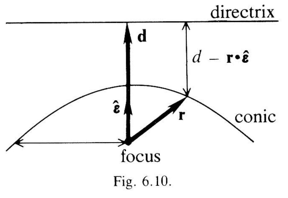
Fig. 6.10.
The defining condition for a conic can then be written
\, \dfrac { | \, \bold r \, | } { d - \bold r \cdot \hat{\boldsymbol{\varepsilon}} } = \varepsilon. \;\;\;\;\;\;\;\;\;\;\;\;\;\;\;\;\;\;\;\;\;\;\;\;\;\;\;\;\;\;\;\;\;\;\;\;\;\;\;\;\;\;\;\;\;\;\;\;\;\;\;\;\;\;\;\;\;\;\;\;\;\;\;\;\;\;\;\;\;\;\;\;\;\;\;\;\; (6.34)
Solving this for \, r = | \, \bold r \, | \, and introducing the eccentricity vector \, \boldsymbol{\varepsilon} = \varepsilon \, \hat{\boldsymbol{\varepsilon}} \, along with the so-called semi-latus rectum \, \ell = \varepsilon \, d , we get the more convenient equation
\, r = \dfrac { \ell } { 1 + \boldsymbol{\varepsilon} \cdot \hat{\bold r} }.\;\;\;\;\;\;\;\;\;\;\;\;\;\;\;\;\;\;\;\;\;\;\;\;\;\;\;\;\;\;\;\;\;\;\;\;\;\;\;\;\;\;\;\;\;\;\;\;\;\;\;\;\;\;\;\;\;\;\;\;\;\;\;\;\;\;\;\;\;\;\;\;\;\;\;\;\; (6.35)
This expresses the distance \, r \, from the focus to a point on the conic as a function of the direction \, \hat{\bold r} \, to the point. Alternatively, the same condition can be expressed as a parametric equation for \, r \, as a function of the angle \, \theta \, between \, \boldsymbol{\varepsilon} \, and \, \hat{\bold r} . Thus, substituting \, \boldsymbol{\varepsilon} \cdot \hat{\bold r} = \varepsilon \, \cos \theta \, into (6.35), we get
\, r = \dfrac { \ell } { 1 + \varepsilon \, \cos \theta }.\;\;\;\;\;\;\;\;\;\;\;\;\;\;\;\;\;\;\;\;\;\;\;\;\;\;\;\;\;\;\;\;\;\;\;\;\;\;\;\;\;\;\;\;\;\;\;\;\;\;\;\;\;\;\;\;\;\;\;\;\;\;\;\;\;\;\;\;\;\;\;\;\; (6.36)
This is a standard equation for conics, but we usually prefer (6.35), because it shows the dependence of \, r \, on the directions \, \hat{\boldsymbol{\varepsilon}} \, and \, \hat{\bold r} \, explicitly, while this dependence in (6.36) is expressed only indirectly through the definition of \, \theta .
Equation (6.35) determines a curve when \, r \, is restricted to directions in a plane, but if \, r \, is allowed to range over all directions of \, {\mathscr{E}}_3 \, , then (6.35) describes a 2-dimensional surface called a conicoid. Our definition of a conic can be used for a conicoid simply by interpreting the directrix as a plane instead of a line. Both the conics and the conicoids are classified according to the values of the eccentricity shown in Table 6.1.
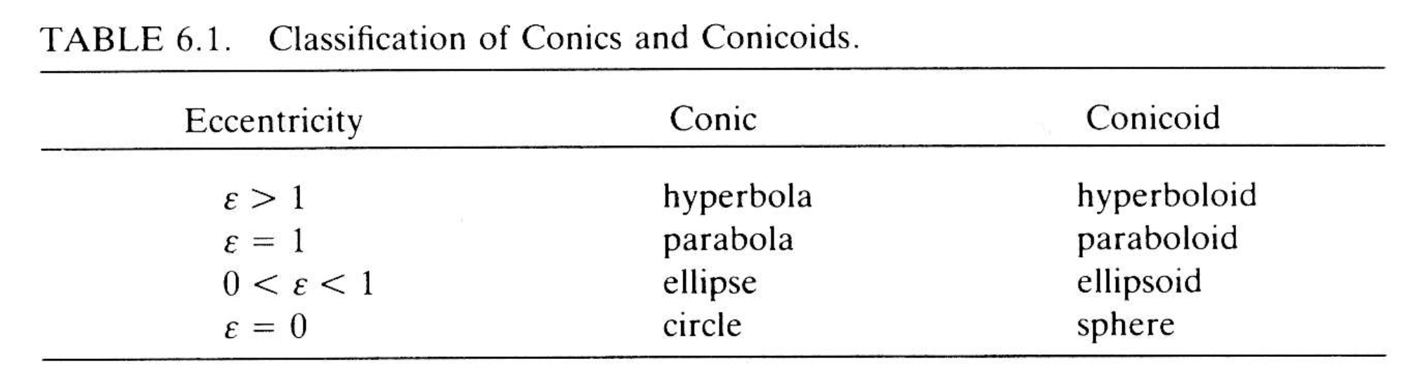
Table 6.1.
The 1-parameter family of conics with a common focus and pericenter is illustrated in Figure 6.11. The pericenter is the point on the conic at which \, r \, has a minimum value. In the hyperbolic case there are actually two pericenters, one on each branch of the hyperbola. Only one of these is shown in Figure 6.11. If the conics in Figure 6.11 are rotated about the axis through the focus and the pericenter, they sweep out the corresponding conicoids.

Fig. 6.11 Conics with a common focus and pericenter
The conics and the conicoids have quite a remarkable variety of properties, which is related to the fact that they can be described by many different equations besides (6.35). Rather than undertake a systematic study of those properties, we shall wait for them to arise in the context of physical problems, and we will be better prepared for this when we have the tools of differential calculus at our disposal.
Our study of analytic geometry has just begun. The study of particle trajectories, which we undertake in the next chapter, is largely analytic geometry in \, {\mathscr{E}}_3 . For those who wish to study the analytic geometry in \, {\mathscr{E}}_2 \, in more detail, the book of Zwikker (1963) is recommended. He formulates analytic geometry in terms of complex numbers and shows how much this improves on the traditional methods of coordinate geometry. Of course, everything he does is easily reexpressed in the language of geometric algebra, which has all the advantages of complex numbers and more.
Indeed, geometric algebra brings further improvements to Zwikker’s treatment by enlarging the algebraic system from \, {\mathscr{G}}_2^+ \, to \, {\mathscr{G}}_2 , and so introducing the fundamental distinction between vectors and spinors and along with it the concepts of inner and outer products. Most important, geometric algebra provides for the generalization of the geometry in \, {\mathscr{E}}_2 \, to \, {\mathscr{E}}_3 . The present book develops all the principles and techniques needed for analytic geometry, but Zwikker’s book is a valuable storehouse of particular facts about curves in \, {\mathscr{E}}_2 . Among other things, it includes the remarkable proof that conic sections as defined by (6.34) really are sections of a cone.
/// FORTSÄTT HÄR
/////// End of quote from Hestenes