This page is a sub-page of our page on Mathematical Concepts.
///////
Related KMR-pages:
• Abductive PseudoInverse
• Artificial Ethics
• Digital Bolshevism
• Oscar Reutersvärd
• M.C. Escher
• Disambiguation
• Entropy
• Function
• Homology and Cohomology
• Homotopy
• Space
• Time
• Quotients
• Duality
• Topology
• Dimension
In Swedish:
• Osäkerhetskalkyl
• Förändringskalkyl
///////
Other relevant sources of information:
• The Theory That Would Not Die by Sharon Bertsch McGrayne, Yale University Press, 2011.
• Frequentist probability at Wikipedia.
• Frequentist inference at Wikipedia
• Bayesian probability at Wikipedia.
• Bayesian inference at Wikipedia.
• Bayes theorem, the geometry of changing beliefs by Steven Strogatz on YouTube.
• Probability – The Logic of Science by E.T. Jaynes.
• Convergence of random variables at Wikipedia.
• Convergence of Binomial to Normal: Multiple Proofs, by Subhash Bagui and K.L. Mehra.
• Uncertainty as Applied to Measurements and Calculations by John Denker.
• History of probability at Wikipedia.
• History of statistics at Wikipedia
• The Method of Least Squares at Wikipedia
///////
Uncertainty theory is concerned with modeling the uncertainties in the streams of information that we interact with in a multitupde of different ways. Philosophically speaking uncertainty theory regards the concept of uncertainty from two different and historically antagonistic perspectives:
The frequentist approach is based on computing probabilities
for the appearance of different effects of a given combination of events,
while the bayesian approach is based on computing plausibilities
for their possible causes.
Unfortunately, in most cases the two concepts “frequentist probability” and “bayesian plausibility” are referred to by the overall term of “probability” – for example in the wikipedia link on bayesian “probability” given in the preceeding paragraph under the label “plausibilities.” Sadly, this linguistic homonym contributes to the obfuscation of the temporal difference between these two complementary perspectives on uncertainty.
In summary:
Frequentism computes forward uncertainties
in terms of probabilities for effects.
Bayesianism computes backward uncertainties
in terms of plausibilities for causes.
Hence, frequentism makes use of deductive reasoning, in dealing with probable effects.
while bayesianism makes use of abductive reasoning in dealing with plausible causes.
The effect-probability-based approach leads to frequentist probability theory, frequentism, with its random variables, its possibility spaces, and its assumption of the convergence of the ratio between the number of appearances of a certain event, and the total number of trials in trying to produce it, towards the probability for the occurrence of that event – through a limit when the number of trials are increased beyond any finite bound. This assumption of the convergence of frequency ratios towards probabilities for the occurrence of events is an important axiom of frequentism.
The cause-plausibility-based approach leads to bayesian plausibility theory, bayesianism, which has an objective and a subjective part. Objective bayesianism is concerned with the logic of science itself based on plausible reasoning. Subjective bayesianism, or bayesian inference, is about past histories of inferred plausibilities and different choices carried out based on them, entities that can often be computed by making use of Bayes’ theorem. An excellent visualization of Bayes’ theorem which is making plausibility intuitive is provided by Steven Strogatz on YouTube.
A great advantage of bayesian analysis is the fact that it does not need the possibility spaces of the frequentist theory, nor its effect probabilities. This makes it possible for the bayesian “plausibility engineers” to update their computed plausibilites via experimental observations. Such experimental updates form the basis for so-called machine learning,
a field that is more broadly referred to as artificial intelligence.
Sharon Bertsch McGrayne starts her historical thriller The Theory That Would Not Die – How Bayes’ Rule Cracked the Enigma Code, Hunted Down Russian Submarines, and Emerged Triumphant from Two Centuries of Controversy, with the following quote from the British economist John Maynard Keynes:
When the facts change, I change my opinion. What do you do, sir?
As we have discussed above, both frequentist probability and bayesian plausibility are normally referred to as “probability”. In order to increase the semantic precision of the terms involved in describing uncertainty it is important to distinguish between the meaning of “probability” and “plausibility“.
For example, one can experience it as “highly plausible” that one will be run over by a car if one runs straight out into a road with intensive traffic, but it can never be “highly probable” since there is no frequency quotient – and hence no probability – that can be assigned to such an event.
The history of uncertainty calculus
The development of uncertainty calculus will be described below in a number of different steps that are not strictly chronologically ordered.
•) Games about money have been around for thousands of years but before the time of the Italian mathematician (and enthusiastic gambler) Girolamo Cardano (1501 – 1576) “game theory” was based purely on intuition and guesses. Cardano started to write his book Liber de Ludo Aleae (The Book on Games of Chance) – which dealt with what was later to be called “probabilities” – before he was thirty but didn’t finish it until he had passed sixty. The book was published in 1563 and it presented the first attempt towards a mathematical theory of games. In it Cardano introduce a fractional number between 0 and 1 to represent the concept of probability for different outcomes when throwing dice and showed how to compute the probability of getting either a five or a six when throwing one dice, as well as the probability of getting two sixes when throwing two dice.
Cardano was a polymath who was active within a number of different fields. For example, he invented the cardan shaft which is still being used as a drive shaft in present day vehicles. However, he is most well-known for his revolutionary book about algebra, Ars Magna (The Great Art), from 1545. It describes how one can solve a cubic equation as well as a quartic equation, a process that involves the use of certain “imaginary” entities that several hundred years later became known as complex numbers. Ars Magna was also the first book that made systematic use of negative numbers.
•) The correspondence between Fermat and Pascal
•) The Swiss mathematician Jacob Bernoulli (1655 – 1705) computed averages of combinations of known probabilities for different outcomes of a given game. If the game was interrupted prematurely, Bernoulli’s computations made it possible to divide the “game pot” in a rational way – assuming that both players were judged to be equally skilled, that is, each of them was judged to have a 50% chance of winning.
The law of large numbers is a theorem of probability theory which says that the arithmetic mean of a large number of independent observations of a random variable with increasing probability (towards 1) lies closer and closer to the expected value of the random variable. The law of large numbers can be said to correspond to the intuitive expression that, under certain conditions, “things even out in the long run.”
The law of large numbers exists in two different forms, the weak form and the strong form. The first version of the law of large numbers was formulated and proved by Jacob Bernoulli at the beginning of the eighteenth century, but the proof was not published until his book Ars Conjectandi which was published by his nephew in 1713, eight years after Bernoulli’s death.
What Bernoulli proved in his book corresponds to the weak form of the law for the case where the participating random variables only assume two different values, a so-called
binomial distribution, another concept that was introduced in Bernoulli’s book.
In fact Bernoulli formulated the law of large numbers “in reverse” compared to how this law is usually formulated today: given an outcome from \, n \, trials, how can we determine the expected value. In Bernoulli’s formulation: If we draw \, n \, balls from an urn with only black or white balls, what can be said about the total distribution of the two kinds of balls?
The law of large numbers was given its present formulation in 1933 by Andrei Kolmogorov in his pioneering work Foundations of the Theory of Probability, which laid an axiomatic foundation for the frequentist theory of probability. With his probability axioms Kolmogorov based his probability theory on measure theory – through the axiomatically introduced concept of a sigma algebra.
•) Abraham de Moivre (1667 – 1754) introduced the concepts of sample spaces and random variables. He also introduced the concept of outcome probability for the discrete probability distribution known as the binomial distribution, which can be described as the outcome distribution when one tosses a coin with the probabilities \, \frac {1}{2} \, for heads and \, \frac {1}{2} \, for tails.
In 1718 de Moivre published these results in his book The Doctrine of Chances which laid a mathematical foundation for probability theory. This was the beginning of the idea of convergence in probability.
/////// Quoting Convergence of Binomial to Normal: Multiple Proofs:
It is well known […] that if both \, np \, and \, nq \, are greater than \, 5 , then the binomial probabilities given by the probability mass function (pmf) can be satisfactorily approximated by the corresponding normal [probabilities of the] probability density function (pdf). These approximations […] turn out to be fairly close for \, n \, as low as \, 10 \, when \, p \, is in a neighborhood of \, \frac {1}{2} .
/////// End of quote from “Convergence of Binomial to Normal: Multiple Proofs.”
It is this convergence that makes the prickly curves of the binomial distribution softer and softer as the number of coin tosses increases.
In 1738 de Moivre was the first to suggest the approximation of the binomial distribution by a normal distribution when \, n \, is large. The reasoning behind this proposal was based on Stirling’s approximation.
In 1733 de Moivre used the binomial distribution as an approximation and claimed that when one carries out an unboundedly-increasing number of independent coin-tossing experiments (with the same number of coin tosses in each experiment), the binomial distribution converges towards a limiting distribution (a.k.a an asymptotic distribution). Today this limiting distribution is known as a normal distribution.
In 1812 de Moivre’s results were expanded by Laplace who used the normal distribution to approximate the binomial distribution. The de Moivre-Laplace theorem was the first example – and a special case – of one of the most important theorems of probability theory: the central limit theorem.
/////// Quoting Wikipedia:
Dutch mathematician Henk Tijms writes:[41]
“The central limit theorem has an interesting history. The first version of this theorem was postulated by the French-born mathematician Abraham de Moivre who, in a remarkable article published in 1733, used the normal distribution to approximate the distribution of the number of heads resulting from many tosses of a fair coin.
This finding was far ahead of its time, and was nearly forgotten until the famous French mathematician Pierre-Simon, marquis de Laplace rescued it from obscurity in his monumental work Théorie analytique des probabilités, which was published in 1812. Laplace expanded De Moivre’s finding by approximating the binomial distribution with the normal distribution.
But as with de Moivre, Laplace’s finding received little attention in his own time. It was not until the nineteenth century was at an end that the importance of the central limit theorem was discerned, when, in 1901, Russian mathematician Aleksandr Lyapunov defined it in general terms and proved precisely how it worked mathematically. Nowadays, the central limit theorem is considered to be the unofficial sovereign of probability theory.”
Sir Francis Galton described the Central Limit Theorem in this way:[42]
“I know of scarcely anything so apt to impress the imagination as the wonderful form of cosmic order expressed by the “Law of Frequency of Error“. The law would have been personified by the Greeks and deified, if they had known of it. It reigns with serenity and in complete self-effacement, amidst the wildest confusion. The huger the mob, and the greater the apparent anarchy, the more perfect is its sway. It is the supreme law of Unreason. Whenever a large sample of chaotic elements are taken in hand and marshalled in the order of their magnitude, an unsuspected and most beautiful form of regularity proves to have been latent all along.”
The actual term “central limit theorem” (in German: “zentraler Grenzwertsatz“) was first used by George Pólya in 1920 in the title of a paper.[43][44] Pólya referred to the theorem as “central” due to its importance in probability theory. According to Le Cam, the French school of probability interprets the word central in the sense that “it describes the behaviour of the centre of the distribution as opposed to its tails”.[44] The abstract of the paper On the central limit theorem of calculus of probability and the problem of moments by Pólya[43] in 1920 translates as follows:
“The occurrence of the Gaussian probability density \, e^{-x^2} \, in repeated experiments, in errors of measurements, which result in the combination of very many and very small elementary errors, in diffusion processes etc., can be explained, as is well-known, by the very same limit theorem, which plays a central role in the calculus of probability. The actual discoverer of this limit theorem is to be named Laplace; it is likely that its rigorous proof was first given by Tschebyscheff and its sharpest formulation can be found, as far as I am aware of, in an article by Liapounoff.”
/////// End of quote from Wikipedia
•) Thomas Simpson turned probability calculus around and concentrated on summing the probabilities for error measurements – instead of the probabilities for correct measurements (which leads to averages). Via Carl-Friedrich Gauss this led to the method of least squares for the minimization of the sum of the sum total of the errors of measurement. This extremely useful result is usually attributed to Gauss, but it was actually first published by Adrien-Marie Legendre.
•) Thomas Bayes (1701 – 1761) found a very clever way to compute the necessary plausibilities for the bayesian approach to statistics. He made use of the theorem that carries his name (Bayes’ theorem) and which was not published until after his death.
•) Pierre-Simon Laplace (1749 – 1827) developed and popularized both the frequentist and the bayesian forms of statistics as well as many other important parts of mathematics. Laplace was one of the leading mathematicians of his time and his Celestial Mechanics (in five volumes) expanded on Newton’s ideas from his Principia of 1687, using Leibniz’ version of the infinitesimal calculus as well as his own extensions to this calculus.
Together with mathematicians such as Leonard Euler, Joseph-Louis Lagrange, Peter Gustav Lejeune Dirchlet and Siméon Denis Poisson, Laplace contributed to the development of a number of important tools to help solve partial differential equations, such as the calculus of variations and Laplace transform, as well as the technique that uses so-called generating functions. One of the most important partial differential equations in physics goes by the name of Laplace’s equation since Laplace was the first person to study it.
/////// Quoting Wikipedia:
In probability theory, the central limit theorem (CLT) establishes that, in some situations, when independent random variables are added, their properly normalized sum tends toward a normal distribution (informally a “bell curve”) even if the original variables themselves are not normally distributed. The theorem is a key concept in probability theory because it implies that probabilistic and statistical methods that work for normal distributions can be applicable to many problems involving other types of distributions.
For example, suppose that a sample is obtained containing a large number of observations, each observation being randomly generated in a way that does not depend on the values of the other observations, and that the arithmetic mean of the observed values is computed. If this procedure is performed many times, the central limit theorem says that the distribution of the average will be closely approximated by a normal distribution. A simple example of this is that if one flips a coin many times the probability of getting a given number of heads in a series of flips will approach a normal curve, with mean equal to half the total number of flips in each series. (In the limit of an infinite number of flips, it will equal a normal curve.)
The central limit theorem has a number of variants. In its common form, the random variables must be identically distributed. In variants, convergence of the mean to the normal distribution also occurs for non-identical distributions or for non-independent observations, given that they comply with certain conditions.
The earliest version of this theorem, that the normal distribution may be used as an approximation to the binomial distribution, is now known as the de Moivre–Laplace theorem.
/////// End of quote from Wikipedia
/////// Quoting Investopedia:
Understanding the Central Limit Theorem (CLT)
According to the central limit theorem, the mean of a sample of data will be closer to the mean of the overall population in question as the sample size increases, notwithstanding the actual distribution of the data, and whether it is normal or non-normal. This concept was first discovered by Abraham de Moivre in 1733 though it wasn’t named until George Polya, in 1920, dubbed it the Central Limit Theorem.
As a general rule, sample sizes equal to or greater than 30 are considered sufficient for the CLT to hold, meaning the distribution of the sample means is fairly normally distributed. So, the more samples that one takes results in the graph looking more and more like that of a normal distribution.
Another key aspect of CLT is that the average of the sample means and standard deviations will equal the population mean and standard deviation. This is extremely useful in predicting the characteristics of a population with a high degree of accuracy.
Key Takeaways:
• The central limit theorem (CLT) states that the distribution of sample means approximates a normal distribution as the sample size gets larger.
• Sample sizes equal to or greater than 30 are considered sufficient for the CLT to hold.
• A key aspect of CLT is that the average of the sample means and standard deviations will equal the population mean and standard deviation.
• A sufficiently large sample size can predict the characteristics of a population accurately.
/////// End of quote from Investopedia
/// INTRO TEXT HERE
(ii) The Law of Large Numbers
(iii) The Central Limit Theorem.
• Random variable
• Cumulative Distribution Function
• Probability Density Function
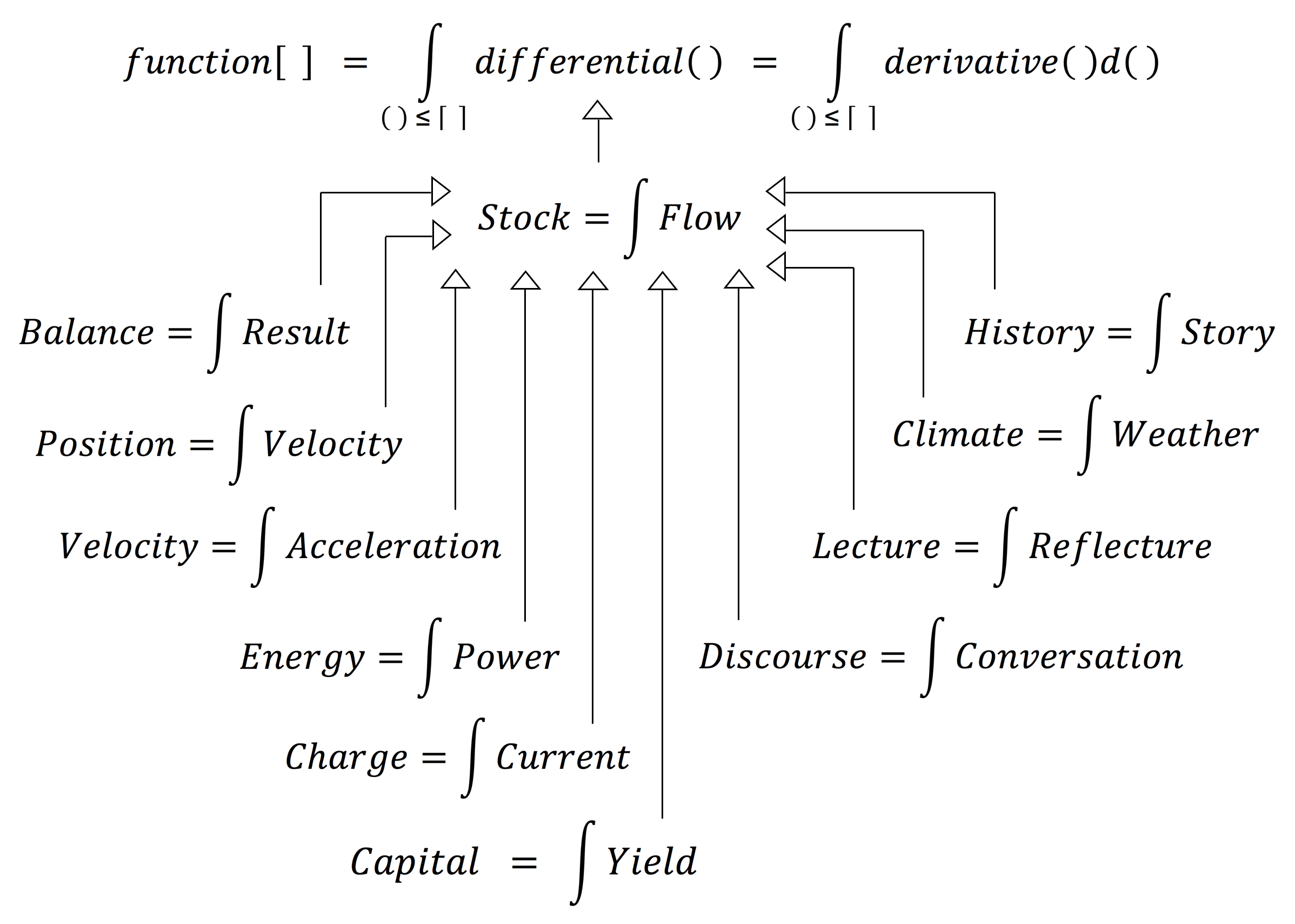
The cumulative distribution function (CDF) and the probability distribution function (PDF) are related as antiderivative and derivative by the fundamental theorem of calculus.
This theorem can be formulated in the following formula-free way:
The derivative
of any antiderivative
of a continuous function
is equal to the function itself.
By applying this theorem to probability theory we get:
The CDF is an antiderivative of the PDF,
and the PDF is the derivative of the CDF.
and therefore
For a continuous function f
The derivative of its CDF
is equal to its PDF.
NOTE: The PDF of f is equal to f itself.
Or, in plain text:
The derivative of the cumulative distribution of a random variable
is equal to the probability distribution of the variable,
which is also referred to as the density of the variable.
NOTE: The role of the “function” is here played by the “random variable.”
///////
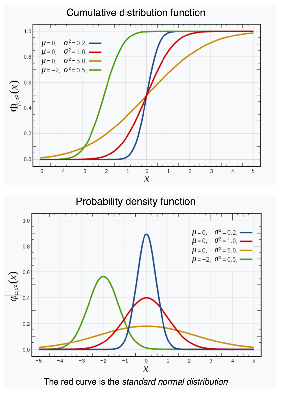
Image source: https://en.wikipedia.org/wiki/Normal_distribution
///////
(1): The value \, F(x) \, of the cumulative distribution \, F \, for a random variable at a point \, x
represents the probability that the random variable assumes a value
that is less than or equal to \, x .
(2): The value \, f(x) \, of the probability distribution \, f \, for a random variable at a point \, x
is proportional to the probability that the random variable assumes a value
that lies within an infinitesimal (= “infinitely small”) interval \, dx \, around the point \, x .
NOTE: If \, x \, is a real number, such an interval \, dx \, does not exist. This criticism was voiced by George Berkely (1685 – 1753), who accused the followers of Newton and Leibniz of “computing with the ghosts of departed quantities.”
/// Describe the “wild computations” of the 1700s and the clarification, in the 1800s, of the reasons behind such errors – leading to a stringent limit-based approach to infinitesimals developed by Karl Weierstrass (and his school).
However, in the early 1960s, Abraham Robinson introduced an extension of calculus called nonstandard analysis which is based on so-called hyperreal numbers. Among hyperreal numbers infinitesimals actually exist and can be computed with just like real numbers.
///////
Some of the applications of the fundamental theorem of calculus :
///////
Summary:
The law of large numbers states that the arithmetic mean value
of many statistically independent observations of a random variable
with large probability lies close to the varible’s expected value.
The central limit theorem states that the distribution of averages
of a a boundlessly increasing number of trials ALWAYS “becomes” normal,
even if the distribution of averages in each of these trial is not necessarily normal.
When computing the expected value of a sum of independent and equally distributed random variables, and when either the number of random variables in each trial increases, or the number of trials increases, these two fundamental statistical “forces” create a convergence of the expected value of the sum towards a normal distribution, described by a bell curve)
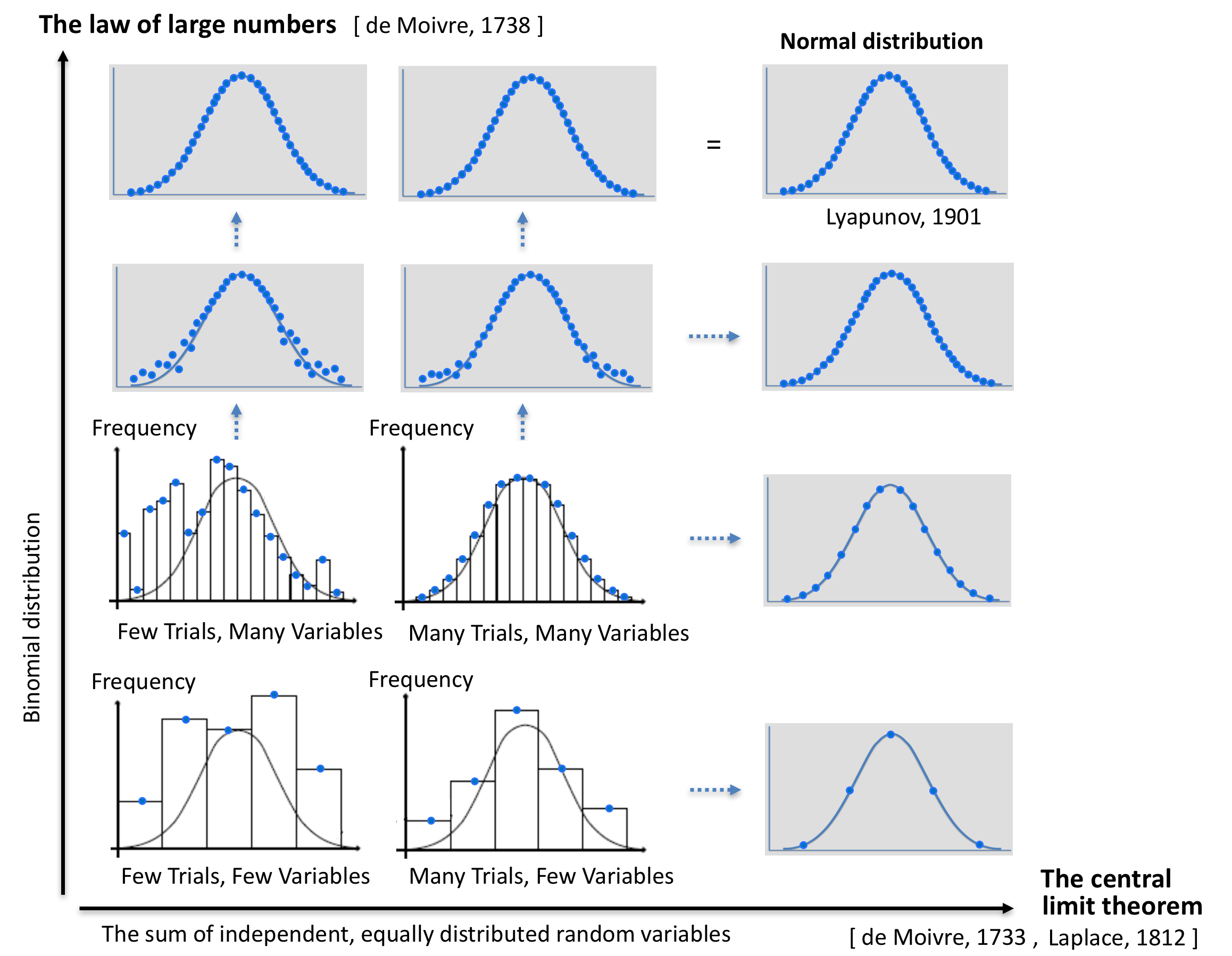
Based on a diagram från Mathematics illuminated: Making Sense of Randomness.
How these structures can be utilized in order to create better understanding and better analyzes of statistics in sports is described at the website Tabmathletics.
///////
Properties of the normal distribution
Cumulative Distribution Function (CDF) of the normal distribution
Cramér’s decomposition theorem is equivalent to saying that
the convolution of two distributions is normal if and only if both are normal.
Cramér’s decomposition theorem implies that
a linear combination of independent non-Gaussian random variables
will never have an exactly normal distribution,
although it may approach it arbitrarily closely.
///////