This page is a sub-page of our page on New Foundations for Classical Mechanics.
///////
Related KMR-pages:
• Chapter 1: Origins of Geometric Algebra
• Chapter 2: Developments in Geometric Algebra
• Chapter 3: Mechanics of a Single Particle
///////
Books:
• René Descartes (1637), La Géometrie
• Hermann Günther Graßmann (1844), Die Lineale Ausdehnungslehre, ein neuer Zweig der Mathematik
• A New Branch Of Mathematics – The Ausdehnungslehre of 1844 and Other Works, translated by Lloyd C. Kannenberg (1995)
• William Kingdon Clifford (1878), Applications of Grassmann’s Extensive Algebra, American Journal of Mathematics Vol. 1, No. 4 (1878), pp. 350-358 (9 pages), Published by: The Johns Hopkins University Press
• David Hestenes (1993, (1986)), New Foundations for Classical Mechanics
///////
Other relevant sources of information:
/////// TEMPORARY BEGIN:
\, L_x \; L_y \; \textcolor{red}{L} \, .
\, {\textcolor{red}{L}}^2 = L_x^2 + L_y^2 \, .
\, x \; y \; z \; A_{xy} \; A_{xz} \; A_{yz} \; \textcolor{red}{A} \, .
\, {\textcolor{red}{A}}^2 = {A_{xy}}^2 + {A_{xz}}^2 + {A_{yz}}^2 \, .
\, \hat{\bold a} \hat{\bold b} = e^{\, \bold C} = \cos C + \hat{\bold C} \sin C \, .
\, \hat{\bold b} \hat{\bold c} = e^{\, \bold A} = \cos A + \hat{ \bold A} \sin A \, .
\, \hat{\bold c} \hat{\bold a} = e^{\, \bold B} = \cos B + \hat{\bold B} \sin B \, .
///////
\, \hat{\bold B} \hat{\bold A} = e^{\, i \bold c} = \cos c + i \hat{\bold c} \sin c \, .
\, \hat{\bold C} \hat{\bold B} = e^{\, i \bold a} = \cos a + i \hat{\bold a} \sin a \, .
\, \hat{\bold A} \hat{\bold C} = e^{\, i \bold b} = \cos b + i \hat{\bold b} \sin b \, .
///////
\, \cos (-C) + \hat{\bold C} \sin (-C) = (\cos A + \hat{ \bold A} \sin A) (\cos B + \hat{\bold B} \sin B) \, .
\, \cos (-C) = \cos A \cos B + \sin A \sin B \hat{ \bold A} \hat{\bold B} \, .
\, \cos C = \cos A \cos B + \sin A \sin B \cos c \, .
///////
\, -\hat{\bold C} \sin C = \hat{ \bold A} \sin A \cos B + \hat{\bold B} \sin B \cos A - i \hat{\bold c} \sin A \sin B \, .
///////
\, \bold A = \hat{\bold A} A \; , \; \bold B = \hat{\bold B} B \; , \; \bold C = \hat{\bold C} C \, .
\, \bold a = \hat{\bold a} a \;\; , \; \bold b = \hat{\bold b} b \;\; , \; \bold c = \hat{\bold c} c \, .
///////
\, {\hat{\bold A}}^2 = {\hat{\bold B}}^2 = {\hat{\bold C}}^2 = -1 \, .
\, {\hat{\bold a}}^2 = {\hat{\bold b}}^2 = {\hat{\bold c}}^2 = 1 \, .
///////
\, \hat{\bold a} \hat{\bold b} \, \hat{\bold b} \hat{\bold c} \, \hat{\bold c} \hat{\bold a} = 1 \, .
\, e^{\, \bold C} e^{\, \bold A} e^{\, \bold B} = 1 \, .
\; e^{ - \bold C} = e^{\,\bold A} e^{\, \bold B} \, .
///////
\, (\hat{\bold B} \hat{\bold A}) \, (\hat{\bold A} \hat{\bold C}) \, (\hat{\bold C} \hat{\bold B}) = -1 \, .
\, e^{\, i \bold c} e^{\, i \bold a} e^{\, i \bold b} = -1 \, .
\, e^{\, -i \bold c} = -e^{\, i \bold a} e^{\, i \bold b} \, .
///////
\, \cos c = -\cos a \cos b + \sin a \sin b \cos C \, .
\, \hat{\bold a} \wedge \hat{\bold b} \wedge \hat{\bold c} \, .
\, \hat{\bold b} \wedge \hat{\bold c} = \hat{\bold A} \, .
\, \hat{\bold a} \wedge \hat{\bold b} \wedge \hat{\bold c} \, = \hat{\bold a} \wedge \hat{\bold A} \sin A = \hat{\bold b} \wedge \hat{\bold B} \sin B = \hat{\bold c} \wedge \hat{\bold C} \sin C .
///////
\, \hat{\bold A} \hat{\bold B} \hat{\bold C} \, .
\, {\lang\hat{\bold A} \hat{\bold B} \hat{\bold C}\rang}_0 = -{\lang\hat{\bold A} i\, \hat{\bold a}\rang}_0 \sin A = -i\,\hat{\bold a}\wedge\hat{\bold A} \sin a \, .
\, i {\lang\hat{\bold A} \hat{\bold B} \hat{\bold C}\rang}_0 = \hat{\bold a}\wedge\hat{\bold A} \sin a = \hat{\bold b}\wedge\hat{\bold B} \sin b = \hat{\bold c}\wedge\hat{\bold C} \sin c \, .
\, \frac {\hat{\bold a} \wedge \hat{\bold b} \wedge \hat{\bold c} } { i {\lang\hat{\bold A} \hat{\bold B} \hat{\bold C}\rang}_0 } = \frac {\sin A} {\sin a} = \frac {\sin B} {\sin b} = \frac {\sin C} {\sin c} \, .
///////
/////// TEMPORARY END
\, \mathrm{ \bold v } ( \mathrm{ \bold u } ) = e^{ \, - { \bold i } \alpha /2 } \, \mathrm{ \bold u } \, e^{ \, { \bold i } \alpha /2 } \, .
\, \mathrm{ \bold w } ( \mathrm{ \bold v } ) = e^{ \, - { \bold j } \beta /2 } \, \mathrm{ \bold v } \, e^{ \, { \bold j } \beta /2 } \, .
///////
\, \mathrm{ \bold {w} } (\mathrm{ \bold {v} } ( \mathrm{ \bold u } ) ) = e^{ \, - { \bold j } \beta /2 } \,e^{ \,- { \bold i } \alpha /2 } \, \mathrm{ \bold u } \, e^{ { \bold i } \alpha /2 } \, e^{ \, { \bold j } \beta /2 } \, .
///////
\, {\text{Rot}}_{ {\bold i } \alpha} ( \mathrm{ \bold u} ) = \mathrm{ \bold u} \, e^{ { \bold i } \alpha} \, .
\, \mathrm{ \bold v} = \mathrm{ \bold u} \, e^{ { \bold i } \alpha} \, .
\, {\text{Rot}}_{ {\bold j } \beta } (\mathrm{ \bold v } ) + \mathrm{\bold p} = e^{ \, - \, { \bold j } \beta /2 } \, \mathrm{ \bold u} \, e^{ { \bold i } \alpha} e^{ \, {\bold j } \beta /2 } + \mathrm{ \bold p} \, .
\, \mathrm{ \bold w} = e^{ \, - { \bold j } \beta /2 } \, \mathrm{\bold v} \, e^{ \, { \bold j } \beta /2 } \, .
\, \mathrm{ \bold w} = e^{ \, - { \bold j } \beta /2 } \, \mathrm{ \bold u} e^{ { \bold i } \alpha} \, e^{ \, { \bold j } \beta /2 } \, .
\, \mathrm{ \bold {v} } = \frac{ \mathrm{ \bold {T} } - \mathrm{ {\bold 0} } } { \| \mathrm{ \bold {T} } - \mathrm{ {\bold 0} } \| } \, .
\, \mathrm{ \bold u } \wedge \mathrm{ \bold v } = \| \mathrm{ \bold u } \wedge \mathrm{ \bold v } \| e^{ {\bold i} \alpha } \, .
\, \mathrm{ \bold w } = \frac{ \mathrm{ \bold {T} } - \mathrm{ {\bold P} } } { \| \mathrm{ \bold {T} } - \mathrm{ {\bold P} } \| } \, .
\, \mathrm{ \bold v } \wedge \mathrm{ \bold {w} } = \| \mathrm{ \bold v } \wedge \mathrm{ \bold {w} } \| e^{ \, \bold j \beta } \, .
\, \mathrm{ \bold v } ( \mathrm{ \bold u } ) = e^{ \, - { \bold i } \alpha /2 } \, \mathrm{ \bold u } \, e^{ \, { \bold i } \alpha /2 } \, .
///////
\, R_{ {\bold i} \, \beta/2}( {\bold w} )+\mathrm{P} = e^{ \, - \, { \bold j } \, \beta /2 } \, {\bold w} \, e^{ \, { {\bold j } \, \beta /2 } \, .
\, \mathrm{ \bold {w} } (\mathrm{ \bold {v} } ( \mathrm{ \bold u } ) ) = e^{ \, - { \bold j } \beta /2 } \,e^{ \, - { \bold i } \alpha /2 } \, \mathrm{ \bold u } \, e^{ { \bold i } \alpha /2 } \, e^{ \, { \bold j } \beta /2 } \, .
//////
\, R_{ \bold {i} { \mathrm{ \bold {v} } = \mathrm{ \bold {u} } \, e^{ { \bold i } \, \alpha }\, .
\, \mathrm{ \bold {w} } (\mathrm{ \bold {v} } ) = e^{ \, - \, { \bold j } \, \beta /2 } \, \mathrm{ \bold {v} } \, e^{ \, { \bold j } \, \beta /2 } \, .
\, \mathrm{ \bold {w} } = \mathrm{ \bold {v} } \, e^{ { \, \bold j } \, \beta }\, .
\, \mathrm{ \bold {w} } (\mathrm{ \bold {v} } ( \mathrm{ \bold {u} } ) ) = e^{ \, - \, { \bold j } \, \beta /2 } \,e^{ \, - \, { \bold i } \, \alpha /2 } \, \mathrm{ \bold {u} } \, e^{ \, { \bold i } \, \alpha /2 } \, e^{ \, { \bold j } \, \beta /2 } \, .
\, \mathrm{ \bold {w} } = \mathrm{ \bold {u} } \, e^{ {\bold i } \, \alpha } e^{ { \, \bold j } \, \beta } \, .
/////////////////////
\, \hat{\bold r} = \hat{\boldsymbol{\varepsilon}} \, e^{ \, \bold i \, \theta }, \;\;\;\;\;\;\;\;\;\;\;\;\;\;\;\;\;\;\;\;\;\;\;\;\;\;\;\;\;\;\;\;\;\;\;\;\;\;\;\;\;\;\;\;\;\;\;\;\;\;\;\;\;\;\;\;\;\;\;\;\;\;\;\;\;\;\;\;\;\;\;\;\;\;\;\;\;\;\;\;\; (1.15)
///////
/////// Quoting Hestenes: New Foundations for Classical Mechanics (Chapter 4)
Chapter 4. Central Forces and Two-Particle Systems
///////
Table Of Content
4-1. Angular Momentum
4-2. Dynamics from Kinematics
4-3. The Kepler Problem
///////
The simple laws of force studied in Chapter 3 are said to be phenomenological laws, which is to say that they are only ad hoc or approximate descriptions of real forces in nature. As a rule, they describe resultants of forces exerted by a very large number of particles. A fundamental force law describes the force exerted by a single particle. The simplest candidates for such a law are central forces with the particle at the center of force. This is reason enough for the systematic study of central forces in this chapter. And it should be no surprise that the results are of great practical value.
The investigation of fundamental forces is actually a two-particle problem, for, as Newton’s third law avers, a particle cannot act without being acted upon. Fortunately, the two-particle central force problem can be reduced to a mathematically equivalent one-particle problem, greatly simplifying the solution. However, a complete description of central force motion must include an account of the “two-body effects” involved in this reduction.
4-1. Angular Momentum
We have seen that motion of a particle in any conservative force field is characterized by a conserved quantity called energy. Now we shall show that general motion in a central force field is characterized by another conserved quantity called angular momentum. Then we shall derive properties of angular momentum which will be helpful in a detailed analysis of central force motion.
A force field \, \bold f = \bold f (\bold x) \, is said to be central if it is everywhere directed along a line through a fixed point \, \bold x' \, called the center of force. This property can be expressed by the equation
\, (\bold x -\bold x') \wedge \bold f = \bold r \wedge \bold f = 0 \, \;\;\;\;\;\;\;\;\;\;\;\;\;\;\;\;\;\;\;\;\;\;\;\;\;\;\;\;\;\;\;\;\;\;\;\;\;\;\;\;\;\;\;\;\;\;\;\;\;\;\;\;\;\;\;\;\;\;\;\; (1.1)
where \, \bold r = \bold x -\bold x' \, is introduced as a convenient position variable with the center of force as origin. The angular momentum \, \bold L \, about the center of force for a particle with mass \, m \, is defined by
\, \bold L \equiv m \, \bold r \wedge \dot{\bold r} = m \, (\bold x -\bold x') \wedge \dot{\bold x} \, \;\;\;\;\;\;\;\;\;\;\;\;\;\;\;\;\;\;\;\;\;\;\;\;\;\;\;\;\;\;\;\;\;\;\;\;\;\;\;\;\;\;\;\;\;\;\;\;\;\;\; (1.2)
It is customary to define the angular momentum as a vector quantity
\, \bold l \equiv m \, \bold r \times \dot{\bold r} \, \;\;\;\;\;\;\;\;\;\;\;\;\;\;\;\;\;\;\;\;\;\;\;\;\;\;\;\;\;\;\;\;\;\;\;\;\;\;\;\;\;\;\;\;\;\;\;\;\;\;\;\;\;\;\;\;\;\;\;\;\;\;\;\;\;\;\;\;\;\;\;\;\;\;\;\;\;\;\; (1.3)
However, the bivector \, \bold L \, is more fundamental than the vector \, \bold l \, and will be somewhat more convenient in our study of central forces. In any case, it is easy to switch from one quantity to the other, because they are related by duality; specifically
\, \bold L = i \, \bold l. \;\;\;\;\;\;\;\;\;\;\;\;\;\;\;\;\;\;\;\;\;\;\;\;\;\;\;\;\;\;\;\;\;\;\;\;\;\;\;\;\;\;\;\;\;\;\;\;\;\;\;\;\;\;\;\;\;\;\;\;\;\;\;\;\;\;\;\;\;\;\;\;\;\;\;\;\;\;\;\;\;\;\;\;\;\; (1.4)
We shall use the term angular momentum for either \, \bold L \, or \, \bold l \, and add the term “bivector” or “vector” if it is necessary to specify one or the other.
Now, from the equation of motion we have \, \bold r \wedge \bold f = \bold r \wedge m \, \ddot {\bold r} = \frac{d}{dt} ( m \bold r \wedge \dot {\bold r} ) ,
because \, \dot{\bold r} \wedge \dot{\bold r} = 0 . Hence,
\, \bold r \wedge \bold f = 0 \;\;\; if and only if \;\;\; \dot{\bold L} = 0, \;\;\;\;\;\;\;\;\;\;\;\;\;\;\;\;\;\;\;\;\;\;\;\;\;\;\;\;\;\;\;\;\;\;\;\;\;\;\;\;\;\;\;\;\;\;\;\;\;\;\; (1.5)
that is, angular momentum is conserved if and only if the force is central. It should be noted that this conclusion holds even if the force is velocity dependent, though central forces of this type are not common enough to merit special attention here.
Angular momentum has a simple geometrical interpretation. According to Equation (2-8.26), the directed area \, \bold A = \bold A (t) \, swept out by the radius vector \, \bold r \, in time \, t \, is given by
\, \bold A (t) = \frac{1}{2} \int\limits_{\bold r(0)}^{\bold r(t)} \bold r \wedge d \bold r = \frac{1}{2} \int\limits_{0}^{t} \bold r \wedge \dot{\bold r} \, dt. \;\;\;\;\;\;\;\;\;\;\;\;\;\;\;\;\;\;\;\;\;\;\;\;\;\;\;\;\;\;\;\;\;\;\;\;\;\;\;\;\;\;\;\;\; (1.6)
Therefore, the rate at which area is swept out is determined by the angular momentum according to
\, \bold {\dot{A}} = \frac{1}{2} \, \bold r \wedge \dot{\bold r} = \dfrac{ \bold L}{ 2m }. \, \;\;\;\;\;\;\;\;\;\;\;\;\;\;\;\;\;\;\;\;\;\;\;\;\;\;\;\;\;\;\;\;\;\;\;\;\;\;\;\;\;\;\;\;\;\;\;\;\;\;\;\;\;\;\;\;\;\;\;\;\;\;\;\;\;\;\; (1.7)
For constant angular momentum this can be integrated immediately, with the result
\, \bold A (t) = \frac{1}{2m} \bold L \, t. \;\;\;\;\;\;\;\;\;\;\;\;\;\;\;\;\;\;\;\;\;\;\;\;\;\;\;\;\;\;\;\;\;\;\;\;\;\;\;\;\;\;\;\;\;\;\;\;\;\;\;\;\;\;\;\;\;\;\;\;\;\;\;\;\;\;\;\;\;\;\;\;\;\;\;\, (1.8)
Thus, we conclude that the radius vector of a particle in a central force field sweeps out area at a constant rate. This is a generalization of Kepler’s Second Law of planetary motion.
The orbit of a particle in a central field lies in a plane through the center of force with direction given by the angular momentum; for, from (1.2) we deduce that every point \, \bold r \, on the orbit satisfies
\, \bold r \wedge \bold L = 0, \;\;\;\;\;\;\;\;\;\;\;\;\;\;\;\;\;\;\;\;\;\;\;\;\;\;\;\;\;\;\;\;\;\;\;\;\;\;\;\;\;\;\;\;\;\;\;\;\;\;\;\;\;\;\;\;\;\;\;\;\;\;\;\;\;\;\;\;\;\;\;\;\;\;\;\;\;\;\;\;\; (1.9)
which, as we have seen in Section 2-6, is a necessary and sufficient condition for a point \, \bold r \, on the orbit to lie in the \, \bold L -plane.
If the orbit in a central field is closed, then the particle will return to its starting point in a definite time \, T \, called the period of the motion. From (1.6) and (1.8), we conclude that the period is given by
\, \bold A (T) = \frac{1}{2} \oint \bold r \wedge d \bold r = \frac{1}{2m} \bold L \, T. \;\;\;\;\;\;\;\;\;\;\;\;\;\;\;\;\;\;\;\;\;\;\;\;\;\;\;\;\;\;\;\;\;\;\;\;\;\;\;\;\;\;\;\;\;\;\;\;\;\;\;\, (1.10)
As we shall see, this formula leads to Kepler’s third law of planetary motion.
A major reason for the importance of angular momentum is the fact that it determines the rate at which the radius vector changes direction.
To see this, we differentiate \, \bold r = r \, \hat{\bold r} \, to get
\, \dot{\bold r} = \dot{r} \, \hat{\bold r} + r \, \dot{ \hat {\bold r} }. \, \;\;\;\;\;\;\;\;\;\;\;\;\;\;\;\;\;\;\;\;\;\;\;\;\;\;\;\;\;\;\;\;\;\;\;\;\;\;\;\;\;\;\;\;\;\;\;\;\;\;\;\;\;\;\;\;\;\;\;\;\;\;\;\;\;\;\;\;\;\;\;\;\;\;\; (1.11)
Whence,
\, \bold r \wedge \dot{\bold r} = r \, \bold r \wedge \dot{\hat{\bold r} } = r^2 \, \hat{\bold r} \, \dot{\hat{\bold r}}, \;\;\;\;\;\;\;\;\;\;\;\;\;\;\;\;\;\;\;\;\;\;\;\;\;\;\;\;\;\;\;\;\;\;\;\;\;\;\;\;\;\;\;\;\;\;\;\;\;\;\;\;\;\;\;\;\;\;\;\;\, (1.12)
or
\, \dot{\hat{\bold r}} = \dfrac{ \hat{\bold r} \, \bold L }{ m \, r^2} = \dfrac{ \bold r \, \bold L }{ m \, | \, \bold r \, |^3 } = - \dfrac{ \bold L \, \bold r }{ m \, r^3 }. \, \;\;\;\;\;\;\;\;\;\;\;\;\;\;\;\;\;\;\;\;\;\;\;\;\;\;\;\;\;\;\;\;\;\;\;\;\;\;\;\;\;\;\;\;\;\;\;\;\; (1.13)
When \, \bold L \, is constant, this gives \, \dot{\hat{\bold r}} \, as an explicit function of \, \bold r . Substituting (1.13) into (1.11), we get the velocity in the form
\, \dot{\bold r} = \hat{\bold r} \, ( \dot{r} + \dfrac{ \bold L }{ m \, r } ) = ( \dot{r} - \dfrac{ \bold L }{ m \, r } ) \, \hat{\bold r}. \, \;\;\;\;\;\;\;\;\;\;\;\;\;\;\;\;\;\;\;\;\;\;\;\;\;\;\;\;\;\;\;\;\;\;\;\;\;\;\;\;\;\;\;\;\;\;\;\; (1.14)
For any central force motion, this can be used to determine the velocity as a function of direction \, \dot{\bold r} = \bold v ( \hat{\bold r} ) \, whenever the orbit is expressed as an equation of the form
\, r = r ( \hat{\bold r} ) \, specifying the radial distance as a function of direction.
For planar motion, we can express the radial direction \, \hat{\bold r} \, in the parametric form
\, \hat{\bold r} = \hat{\boldsymbol{\varepsilon}} \, e^{ \, \bold i \, \theta }, \;\;\;\;\;\;\;\;\;\;\;\;\;\;\;\;\;\;\;\;\;\;\;\;\;\;\;\;\;\;\;\;\;\;\;\;\;\;\;\;\;\;\;\;\;\;\;\;\;\;\;\;\;\;\;\;\;\;\;\;\;\;\;\;\;\;\;\;\;\;\;\;\;\;\;\;\;\;\;\;\; (1.15)
where \, \hat{\boldsymbol{\varepsilon}} \, is a fixed unit vector, \, \bold i \equiv \hat{\bold L} \, is the unit bivector for the orbital plane,
and \, \theta = \theta (t) \, is the scalar measure for the angle of rotation.
Differentiating (1.15) and equating to (1.13), we get
\, \dot{\hat{\bold r}} = \hat{\bold r} \, \bold i \, \dot{\theta} = \hat{\bold r} \, \dfrac{ \bold L }{ m \, r^2 } .
So,
\, \bold i \, \dot{\theta} = \dfrac{ \bold L }{ m \, r^2 }. \;\;\;\;\;\;\;\;\;\;\;\;\;\;\;\;\;\;\;\;\;\;\;\;\;\;\;\;\;\;\;\;\;\;\;\;\;\;\;\;\;\;\;\;\;\;\;\;\;\;\;\;\;\;\;\;\;\;\;\;\;\;\;\;\;\;\;\;\;\;\;\;\;\;\;\;\;\;\; (1.16)
Whence
\, L = | \, \bold L \, | = m \, r^2 \, \dot{\theta}. \;\;\;\;\;\;\;\;\;\;\;\;\;\;\;\;\;\;\;\;\;\;\;\;\;\;\;\;\;\;\;\;\;\;\;\;\;\;\;\;\;\;\;\;\;\;\;\;\;\;\;\;\;\;\;\;\;\;\;\;\;\;\;\;\;\;\;\; (1.17)
The derivation of this result assumes only that \, \hat{\bold L} \, is constant. If \, | \, \bold L \, | \, is a constant also, then (1.17) implies that \, \dot{\theta} ≥ 0 \, always, so \, \theta = \theta (t) \, increases monotonically with time if \, | \, \bold L \, | \neq 0 . Therefore, the orbit of a particle in a central field never changes the direction of its circulation about the center of force. We could also have reached this conclusion directly from (1.13).
4-2. Dynamics from Kinematics
The science of motion can be subdivided into kinematics and dynamics. Kinematics is concerned with the description of motion without considering conditions or interactions required to bring particular motions about. Dynamics is concerned with the explanation of motion by specifying forces or other laws of interaction to describe the influence of one physical system on another.
If the dynamics is known, the kinematics of particle motion can be determined by solving the equation of motion. However, the converse problem of determining dynamics from kinematics is far more difficult, and it is rarely solved without considerable prior knowledge about force laws likely to be operative. Historically one of the first and still the most significant solution to such a problem was Newton’s deduction of the law of gravitation from Kepler’s laws. Let us see how the problem can be formulated and solved in modern language.
Kepler’s Laws of Planetary Motion can be formulated as follows:
(1) The planets move in ellipses with the sun at one focus.
(2) The radius vector sweeps out equal areas in equal times.
(3) The square of the period of revolution is proportional to the cube of the semi-major axis.
The first and second laws are illustrated in Figure 2.1; the elliptical orbit is divided into six segments of equal area, showing how a planet’s speed decreases with increasing distance from the sun.
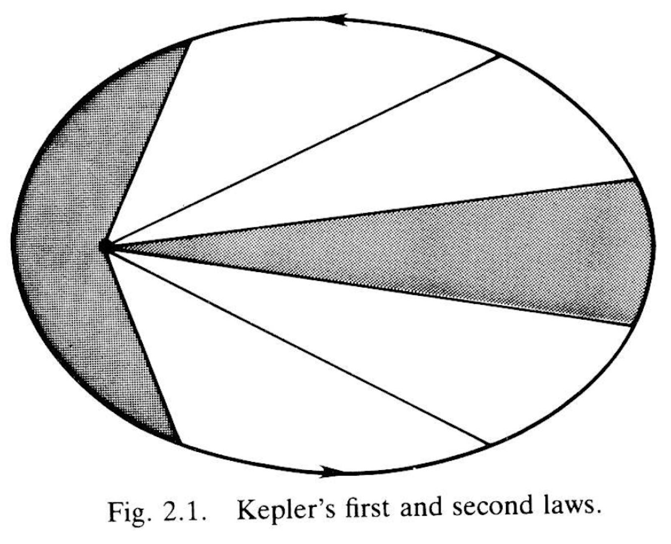
Fig. 2.1. Kepler’s first and second laws
After the discussion in the last section, we recognize Kepler’s second law immediately as a statement of angular momentum conservation, and we conclude that the planets move in a central field with the sun at the center of force. For constant angular momentum, we can compute the acceleration of a particle by using (1.13) to differentiate the expression (1.14) for its velocity; thus
\, \ddot{\bold r} = \dot{\hat{\bold r}} \, ( \dot{r} + \dfrac{ \bold L }{ m \, r } ) + \hat{\bold r} \, ( \ddot{r} - \dfrac{ \dot{r} \, \bold L }{ m \, r^2 } ) = \, \, \;\; = \hat{\bold r} \, [ \, \dfrac{ \bold L }{ m \, r^2 } \, ( \dot{r} + \dfrac{ \bold L }{ m \, r } ) + \ddot{r} - \dfrac{ \dot{r} \, \bold L }{ m \, r^2 } \, ] \,from which we obtain
\, m \, \ddot{\bold r} = ( \, m \, \ddot{r} - \dfrac{ L^2 }{ m \, r^3 } \, ) \, \hat{\bold r} . \;\;\;\;\;\;\;\;\;\;\;\;\;\;\;\;\;\;\;\;\;\;\;\;\;\;\;\;\;\;\;\;\;\;\;\;\;\;\;\;\;\;\;\;\;\;\;\;\;\;\;\;\;\;\;\;\;\;\;\;\;\;\; (2.1)
The right side of this equation has the form of a central force as required, and we can determine the magnitude of of the force by evaluating the coefficient.
Recalling the equation for an ellipse discussed in Section 2-6 (p. 91), we can express Kepler’s first law as an equation of the form
\, r = \dfrac { \ell } { 1 + \boldsymbol{\varepsilon} \cdot \hat{\bold r} }. \;\;\;\;\;\;\;\;\;\;\;\;\;\;\;\;\;\;\;\;\;\;\;\;\;\;\;\;\;\;\;\;\;\;\;\;\;\;\;\;\;\;\;\;\;\;\;\;\;\;\;\;\;\;\;\;\;\;\;\;\;\;\;\;\;\;\;\;\;\;\;\;\;\;\;\;\;\; (2.2)
where \, \ell \, is a positive constant and \, \boldsymbol{\varepsilon} \, is a fixed vector in the orbital plane. As an aid to differentiating (2.2), we multiply (1.13) by \, \varepsilon \, and note that, since \, \boldsymbol{\varepsilon} \wedge \bold L = 0 , the scalar part of the result can be written
\, \boldsymbol{\varepsilon} \cdot \dot{\hat{\bold r}} = \dfrac{ ( \boldsymbol{\varepsilon} \wedge\hat{\bold r} ) \cdot \bold L }{ m \, r^2 } = \dfrac{ \boldsymbol{\varepsilon} \wedge \hat{\bold r} \, \bold L }{ m \, r^2 }, \;\;\;\;\;\;\;\;\;\;\;\;\;\;\;\;\;\;\;\;\;\;\;\;\;\;\;\;\;\;\;\;\;\;\;\;\;\;\;\;\;\;\;\;\;\;\;\;\;\;\;\;\; (2.3a)
while the bivector part has the form
\, \boldsymbol{\varepsilon} \wedge \dot{\hat{\bold r}} = \dfrac{ \boldsymbol{\varepsilon} \cdot \hat{\bold r} \, \bold L }{ m \, r^2 }. \, \;\;\;\;\;\;\;\;\;\;\;\;\;\;\;\;\;\;\;\;\;\;\;\;\;\;\;\;\;\;\;\;\;\;\;\;\;\;\;\;\;\;\;\;\;\;\;\;\;\;\;\;\;\;\;\;\;\;\;\;\;\;\;\;\;\;\;\;\;\;\;\;\; (2.3b)
Now, by differentiating (2.2) we obtain
\, \dot{r} = - \dfrac { \ell \, \boldsymbol{\varepsilon} \cdot \hat{\bold r} } { ( 1 + \boldsymbol{\varepsilon} \cdot \hat{\bold r} )^2 } = - \dfrac { \boldsymbol{\varepsilon} \wedge \hat{\bold r} \, \bold L }{ \ell \, m} .
Differentiating again, we obtain
\, \ddot{r} = - \dfrac{ \boldsymbol{\varepsilon} \cdot \hat{\bold r} \, {\bold L}^2 }{ \ell \, m^2 \, r^2 } = (1 - \dfrac{ \ell }{ r } \, ) \dfrac{ {\bold L}^2 }{ \ell \, m^2 \, r^2 } ,
which, since \, {\bold L}^2 = - L^2 , gives
\, m \, \ddot{r} - \dfrac{ L^2 }{ m \, r^3 } = - \dfrac{ k }{ r^2 }, \;\;\;\;\;\;\;\;\;\;\;\;\;\;\;\;\;\;\;\;\;\;\;\;\;\;\;\;\;\;\;\;\;\;\;\;\;\;\;\;\;\;\;\;\;\;\;\;\;\;\;\;\;\;\;\;\;\;\;\;\;\;\;\;\;\;\;\; (2.4)
where
\, k = \dfrac{ L^2 }{ \ell \, m } > 0. \;\;\;\;\;\;\;\;\;\;\;\;\;\;\;\;\;\;\;\;\;\;\;\;\;\;\;\;\;\;\;\;\;\;\;\;\;\;\;\;\;\;\;\;\;\;\;\;\;\;\;\;\;\;\;\;\;\;\;\;\;\;\;\;\;\;\;\;\;\;\;\;\;\;\;\;\; (2.5)
Comparison of (2.4) with (2.1) leads to the attractive central force law
\, \bold f = - \dfrac{ k \, \hat{\bold r} }{ r^2 }. \;\;\;\;\;\;\;\;\;\;\;\;\;\;\;\;\;\;\;\;\;\;\;\;\;\;\;\;\;\;\;\;\;\;\;\;\;\;\;\;\;\;\;\;\;\;\;\;\;\;\;\;\;\;\;\;\;\;\;\;\;\;\;\;\;\;\;\;\;\;\;\;\;\;\;\;\;\;\;\;\;\; (2.6)
Thus, we have arrived at Newton’s inverse square law for gravitational force. The problem remains to evaluate the constant \, k \, in terms of measurable quantities. Kepler’s third law can be used for this purpose.
According to (1.10) the period \, T \, of a planet’s motion depends on the area enclosed by its orbit. The area integral in (1.10) is most easily evaluated by taking advantage of the fact, proved in Section 2-8, that it is independent of the choice of origin. As we have seen before, with the origin at the center instead of at a focus, an ellipse can be described by the parametric equation
\, \bold x = \bold a \cos \phi + \bold b \sin \phi, \;\;\;\;\;\;\;\;\;\;\;\;\;\;\;\;\;\;\;\;\;\;\;\;\;\;\;\;\;\;\;\;\;\;\;\;\;\;\;\;\;\;\;\;\;\;\;\;\;\;\;\;\;\;\;\;\;\;\;\;\;\;\;\;\; (2.7)
where \, | \, \bold a \, | \, is the semi-major axis referred to in Kepler’s Third Law. Using this to carry out the integration, we get
\, \bold A = \frac{1}{2} \, \oint \bold r \wedge d \bold r = \frac{1}{2} \, \oint \bold x \wedge d \bold x = \, \frac{1}{2} \, \int_0^{2 \pi} \bold x \wedge \dfrac{ d \bold x }{ d \phi } \, d \phi = \pi \bold a \bold b. \;\;\;\;\;\;\;\;\;\; (2.8)
According to (1.10), therefore, the period is given by
\, T = \dfrac{ 2 \pi m \bold a \bold b }{ \bold L } = \dfrac{ 2 \pi m a b }{ L }. \;\;\;\;\;\;\;\;\;\;\;\;\;\;\;\;\;\;\;\;\;\;\;\;\;\;\;\;\;\;\;\;\;\;\;\;\;\;\;\;\;\;\;\;\;\;\;\;\;\;\;\;\;\;\;\;\;\;\;\;\, (2.9)
Squaring this, using (2.5) and the fact that \, b^2 = a \, \ell \, (Exercise (2.2)), we obtain
\, \dfrac { T^2 }{ a^2 } = \dfrac { 4 {\pi}^2 \ell m^2 }{ L^2 } = 4 {\pi}^2 \dfrac { m }{ k }. \;\;\;\;\;\;\;\;\;\;\;\;\;\;\;\;\;\;\;\;\;\;\;\;\;\;\;\;\;\;\;\;\;\;\;\;\;\;\;\;\;\;\;\;\;\;\;\;\;\;\;\;\;\;\;\;\;\;\;\, (2.10)
Kepler’s third law says that this ratio has the same numerical value for all planets. Therefore, the constant \, k \, must be proportional to the mass \, m . Also, note the surprising fact that (2.10) implies that the period \, T \, does not depend on the eccentricity.
Universality of Newton’s Law
We have learned all that Kepler’s laws can tell us about dynamics. Having recognized as much, Newton set about investigating the possibility that the inverse square law (2.6) is a universal law of attraction between all massive particles. He hypothesized that each planet exerts a force on the Sun equal to and opposite to the force exerted by the Sun on the planet. From Kepler’s third law, then, he could conclude that the constant \, k \, is proportional to the mass \, M \, of the Sun as well as the mass \, m \, of the planet, that is
\, k = G m M, \;\;\;\;\;\;\;\;\;\;\;\;\;\;\;\;\;\;\;\;\;\;\;\;\;\;\;\;\;\;\;\;\;\;\;\;\;\;\;\;\;\;\;\;\;\;\;\;\;\;\;\;\;\;\;\;\;\;\;\;\;\;\;\;\;\;\;\;\;\;\;\;\;\;\;\;\;\;\; (2.11)
where \, G \, is a universal constant describing the strength of gravitational attraction between all bodies. Substitution of (2.11) into (2.10) gives
\, M = \dfrac{ 4 {\pi}^2 a^3 }{ G T^2 }. \;\;\;\;\;\;\;\;\;\;\;\;\;\;\;\;\;\;\;\;\;\;\;\;\;\;\;\;\;\;\;\;\;\;\;\;\;\;\;\;\;\;\;\;\;\;\;\;\;\;\;\;\;\;\;\;\;\;\;\;\;\;\;\;\;\;\;\;\;\;\;\;\;\;\;\;\; (2.12)
The constant \, G \, can be determined by measuring the gravitational force between objects on Earth, so (2.12) gives the mass of the Sun from astronomical measurements of \, a \, and \, T .
Kepler presented his three laws as independent empirical propositions about regularities he had observed in planetary motions. He did not possess the conceptual tools needed to recognize that the laws are related to one another, or indeed, to recognize that they are more significant than many other propositions he proposed to describe planetary motion.
Though we have seen how to infer Newton’s universal law of gravitation from Kepler’s laws, and conversely, we can derive all three of Kepler’s laws from Newton’s law, it would be a mistake to think that Newton’s law is merely a summary of information in Kepler’s laws. Actually, Kepler’s laws are only approximately true, and they can be derived only by neglecting the forces exerted by the planets on one another and the Sun. But we shall see that the appropriate corrections can be derived from Newton’s law of gravitation, which is so close to being an exact law of nature that only the most minute deviations from it have been detected. These deviations have been explained only in this century by Einstein’s theory of gravitation.
Epicycles of Ptolemy
Long before Kepler proposed elliptical orbits about the Sun, Ptolemy described the orbits of the planets as epitrochoids centered near the Earth. It is of some interest, therefore, to deduce the force required to produce such a motion.
An epitrochoid is a curve described by the parametric equation
\, \bold r (t) = {\bold r}_1 + {\bold r}_2 = {\bold a}_1 \, e^{i \, {\boldsymbol {\omega}}_1 \, t} + {\bold a}_2 \, e^{i \, {\boldsymbol {\omega}}_2 \, t}, \;\;\;\;\;\;\;\;\;\;\;\;\;\;\;\;\;\;\;\;\;\;\;\;\;\;\;\;\;\;\;\;\;\;\;\;\;\;\;\;\;\;\;\; (2.13)
where
\, {\boldsymbol {\omega}}_1 \wedge {\boldsymbol {\omega}}_2 = 0. \;\;\;\;\;\;\;\;\;\;\;\;\;\;\;\;\;\;\;\;\;\;\;\;\;\;\;\;\;\;\;\;\;\;\;\;\;\;\;\;\;\;\;\;\;\;\;\;\;\;\;\;\;\;\;\;\;\;\;\;\;\;\;\;\;\;\;\;\;\;\;\;\;\;\;\;\;\;\; (2.14)
and \, {\boldsymbol {\omega}}_1 \cdot {\boldsymbol {\omega}}_2 > 0 . If instead \, {\boldsymbol {\omega}}_1 \cdot {\boldsymbol {\omega}}_2 < 0 , the curve is called a hypotrochoid or retrograde epitrochoid. Equation (2.13) is a superposition of two vectors rotating with constant angular velocities in the same plane.
In astronomical literature, the circle generated by one of these vectors is called the epicycle while the circle generated by the other is called the deferrent, and the orbit is traced out by a particle moving uniformly on the epicycle while the center of the epicycle moves uniformly along the deferrent.
A constant vector could be added to (2.13) to express the fact that Ptolemy displaced the center of the planetary orbits slightly from the earth to account for observed variations in speed along the orbits.
Now to deduce the force, we differentiate (2.13) twice; thus
\, \dot{\bold r} = {\boldsymbol {\omega}}_1 \times {\bold r}_1 + {\boldsymbol {\omega}}_2 \times {\bold r}_2 ,
\, \ddot{\bold r} = {\boldsymbol {\omega}}_1 \times ( {\boldsymbol {\omega}}_1 \times {\bold r}_1 ) + {\boldsymbol {\omega}}_2 \times ( {\boldsymbol {\omega}}_2 \times {\bold r}_2 ). \;\;\;\;\;\;\;\;\;\;\;\;\;\;\;\;\;\;\;\;\;\;\;\;\;\;\;\;\;\;\;\;\;\;\;\;\;\;\;\;\; (2.15)
We must eliminate \, {\bold r}_1 \, and \, {\bold r}_2 \, from this last expression to get a force law as a function of \, \bold r \, and \, \dot{\bold r} . To do this, note that
\, ( {\boldsymbol {\omega}}_1 + {\boldsymbol {\omega}}_2 ) \times \, \dot{\bold r} =\, = {\boldsymbol {\omega}}_1 \times ( {\boldsymbol{\omega}}_1 \times {\bold r}_1 ) + {\boldsymbol {\omega}}_2 \times ( {\boldsymbol{\omega}}_2 \times {\bold r}_2 ) - {\boldsymbol{\omega}}_1 \cdot {\boldsymbol{\omega}}_2 \, \bold r + {\boldsymbol {\omega}}_1 \, {\boldsymbol{\omega}}_2 \cdot {\bold r}_1 + {\boldsymbol{\omega}}_2 \, {\boldsymbol{\omega}}_1 \cdot {\bold r}_2 .
But the last two terms vanish when we apply the condition that \, {\bold r}_1 \, and \, {\bold r}_2 \, be orthogonal to a common axis of rotation along \, {\boldsymbol{\omega}}_1 \, and \, {\boldsymbol{\omega}}_2 . Consequently we write (2.15) in the form
\, \ddot{\bold r} = \boldsymbol{\omega} \times \dot{\bold r} + k \, \bold r, \;\;\;\;\;\;\;\;\;\;\;\;\;\;\;\;\;\;\;\;\;\;\;\;\;\;\;\;\;\;\;\;\;\;\;\;\;\;\;\;\;\;\;\;\;\;\;\;\;\;\;\;\;\;\;\;\;\;\;\;\;\;\;\;\;\;\;\;\;\;\;\;\;\, (2.16)
where the vector
\, \boldsymbol{\omega} = {\boldsymbol{\omega}}_1 + {\boldsymbol{\omega}}_2 \;\;\;\;\;\;\;\;\;\;\;\;\;\;\;\;\;\;\;\;\;\;\;\;\;\;\;\;\;\;\;\;\;\;\;\;\;\;\;\;\;\;\;\;\;\;\;\;\;\;\;\;\;\;\;\;\;\;\;\;\;\;\;\;\;\;\;\;\;\;\;\;\;\;\;\;\;\, (2.17a)
and the scalar
\, k = {\boldsymbol{\omega}}_1 \cdot {\boldsymbol{\omega}}_2 \;\;\;\;\;\;\;\;\;\;\;\;\;\;\;\;\;\;\;\;\;\;\;\;\;\;\;\;\;\;\;\;\;\;\;\;\;\;\;\;\;\;\;\;\;\;\;\;\;\;\;\;\;\;\;\;\;\;\;\;\;\;\;\;\;\;\;\;\;\;\;\;\;\;\;\;\;\;\;\; (2.17b)
can be specified independently.
The force law expressed by (2.16) does indeed arise in physical applications, though not from gravitational forces. For \, k < 0 , (2.16) will be recognized as the equation for an isotropic oscillator in a magnetic field, encountered before in Exercise (3-8.5). Equation 2.16 with \, k > 0 \, describes the motion of electrons in the magnetron, a device for generating microwave radiation.
4-3. The Kepler Problem
The problem of describing the motion of a particle subject to a central force varying inversely with the square of the distance from the center of force is commonly referred to as the Kepler Problem. It is the beginning for investigations in atomic theory as well as celestial mechanics, so it deserves to be studied in great detail. Basically, the problem is to solve the equation of motion
\, m \, \ddot{\bold r} = m \, \dot{\bold v} = - \dfrac{k}{r^2} \, \hat{\bold r}. \;\;\;\;\;\;\;\;\;\;\;\;\;\;\;\;\;\;\;\;\;\;\;\;\;\;\;\;\;\;\;\;\;\;\;\;\;\;\;\;\;\;\;\;\;\;\;\;\;\;\;\;\;\;\;\;\;\;\;\;\;\;\;\;\;\;\;\, (3.1)
The “coupling constant” \, k \, depends on the kind of force and describes the strength of interaction. As we saw in the last section, in celestial mechanics the force in (3.1) is Newton’s law of gravitation and \, k = G \, m \, M . IN atomic theory, Equation (3.1) is used to describe the motion of a particle with charge \, q \, in the electric field of a particle with charge \, q' \, ; then \, k = q \, q' , and the force is known as Coulomb’s Law. The Newtownian force is always attractive \, ( k > 0) , whereas the Coulomb force may be either attractive \, ( k > 0) , or repulsive \, ( k < 0) . There are a number of ways to solve Equation (3.1), but the most powerful and insightful method is to determine the constants of motion. We have already seen that angular momentum is conserved by any central force, so we can immediately write down the constant of motion \, \bold L = m \, \bold r \wedge \bold v = m \, r^2 \, \hat{\bold r} \, \dot{\hat{\bold r}}. \;\;\;\;\;\;\;\;\;\;\;\;\;\;\;\;\;\;\;\;\;\;\;\;\;\;\;\;\;\;\;\;\;\;\;\;\;\;\;\;\;\;\;\;\;\;\;\;\;\;\;\;\;\;\;\;\;\;\;\;\;\;\, (3.2) When \, \bold L \neq 0 , we can use this to eliminate \, \hat{\bold r} \, from (3.1) as follows: \, \bold L \, \dot{\bold v} = - \dfrac{ k \, \bold L }{ m \, r^2 } \, \hat{\bold r} = k \, \dot{\hat{\bold r}} . Since \, \bold L \, is constant, this can be written \, \dfrac{d}{dt} (\bold L \, \bold v - k \, \hat{\bold r}) = 0 . Therefore, we can write \, \bold L \, \bold v = k \, (\hat{\bold r} + \boldsymbol{\varepsilon} ), \;\;\;\;\;\;\;\;\;\;\;\;\;\;\;\;\;\;\;\;\;\;\;\;\;\;\;\;\;\;\;\;\;\;\;\;\;\;\;\;\;\;\;\;\;\;\;\;\;\;\;\;\;\;\;\;\;\;\;\;\;\;\;\;\;\;\;\;\;\;\;\;\;\;\, (3.3) where \, \boldsymbol{\varepsilon} \, is a dimensionless constant vector. It should be evident that this new vector constant of motion \, \boldsymbol{\varepsilon} \, is peculiar to the inverse square law, distinguishing it from all other central forces. This constant of motion is called the Laplace vector by astronomers, since Laplace was the first of many to discover it. It is sometimes referred to as the “Runge-Lenz vector” in the physics literature. We shall prefer the descriptive name eccentricity vector suggested by Hamilton.
Since \, \bold L = i \, \bold l , Equation (3.3) can be expressed in terms of the angular momentum vector \,\bold l , with the result
\, \bold v \times \bold l = k \, (\hat{\bold r} + \boldsymbol{\varepsilon}) ,
along with the condition \, \bold l \cdot \bold v = 0 . However, Equation (3.3) is much easier to manipulate, because the geometric product \, \bold L \, \bold v \, is associative while the cross product \, \bold \times \bold v \, is not.
Energy and Eccentricity
Besides \, \bold L \, and \, \boldsymbol{\varepsilon} ,Equation (3.1) conserves energy, for
\, \nabla \, \dfrac{k}{r} = ({\partial}_r \, \dfrac{k}{r} ) \nabla r = - \dfrac{k}{r^2} \, \hat{\bold r} ,
so the force is conservative with potential \, -k r^{-1} . It follows, then, from our general consideration in Section 3-10, that the energy
\, E = \frac{1}{2} m v^2 - \dfrac{k}{r}, \;\;\;\;\;\;\;\;\;\;\;\;\;\;\;\;\;\;\;\;\;\;\;\;\;\;\;\;\;\;\;\;\;\;\;\;\;\;\;\;\;\;\;\;\;\;\;\;\;\;\;\;\;\;\;\;\;\;\;\;\;\;\;\;\;\;\;\;\;\;\;\;\;\;\, (3.4)
is a constant of the motion. However, if \, \bold L \neq 0 , this is not a new constant, because \, E \, is determined by \, \bold L \, and \, \boldsymbol{\varepsilon} . Thus, from (3.3) we have
\, k^2 {\boldsymbol{\varepsilon}}^2 = (\bold L \bold v - k \hat{\bold r})^2 = L^2 v^2 - k ( \bold L \bold v \hat{\bold r} + \hat{\bold r} \bold L \bold v ) + k^2 .
But, by (3.2)
\, ( \bold L \bold v \hat{\bold r} + \hat{\bold r} \bold L \bold v ) = 2 \bold L \bold v \wedge \hat{\bold r} = \dfrac{ 2 \bold L {\bold L}^\dagger }{ m r } = \dfrac{ 2 L^2 }{ m r } .
Hence,
\, k^2 ( {\varepsilon}^2 - 1) = L^2 ( v^2 - \dfrac{ 2 k }{ m r } ) .
The last factor in this equation must be constant, because the other factors are constant. Indeed, using (3.4) to express this factor in terms of energy, we get the relation
\, {\varepsilon}^2 - 1 = \dfrac{ 2 L^2 E }{ m k^2 }. \;\;\;\;\;\;\;\;\;\;\;\;\;\;\;\;\;\;\;\;\;\;\;\;\;\;\;\;\;\;\;\;\;\;\;\;\;\;\;\;\;\;\;\;\;\;\;\;\;\;\;\;\;\;\;\;\;\;\;\;\;\;\;\;\;\;\;\;\;\;\;\;\;\;\, (3.5)
When \, \bold L = 0 , this relation tells us nothing about energy, and our derivation of the energy equation (3,4) from (3.2) and (3.3) fails. But we know from our previous derivation that the energy conservation holds nevertheless. Indeed, for \, \bold L = 0 , Equation (3.2) implies that the orbit lies on a straight line through the origin, and the energy equation (3.4) must be used instead of (3.3) to describe motion along that line.
The Orbit
//// FORTSÄTT HÄR
/////// End of quote from Hestenes (1986)